Now this series on information geometry will take an unexpected turn toward ‘green mathematics’. Lately I’ve been talking about relative entropy. Now I’ll say how this concept shows up in the study of evolution!
That’s an unexpected turn to me, at least. I learned of this connection just two days ago in a conversation with Marc Harper, a mathematician who is a postdoc in bioinformatics at UCLA, working with my friend Chris Lee. I was visiting Chris for a couple of days after attending the thesis defenses of some grad students of mine who just finished up at U.C. Riverside. Marc came by and told me about this paper:
• Marc Harper, Information geometry and evolutionary game theory.
and now I can’t resist telling you.
First of all: what does information theory have to do with biology? Let me start with a very general answer: biology is different from physics because biological systems are packed with information you can’t afford to ignore.
Physicists love to think about systems that take only a little information to describe. So when they get a system that takes a lot of information to describe, they use a trick called ‘statistical mechanics’, where you try to ignore most of this information and focus on a few especially important variables. For example, if you hand a physicist a box of gas, they’ll try to avoid thinking about the state of each atom, and instead focus on a few macroscopic quantities like the volume and total energy. Ironically, the mathematical concept of information arose first here—although they didn’t call it information back then; they called it ‘entropy’. The entropy of a box of gas is precisely the amount of information you’ve decided to forget when you play this trick of focusing on the macroscopic variables. Amazingly, remembering just this—the sheer amount of information you’ve forgotten—can be extremely useful… at least for the systems physicists like best.
But biological systems are different. They store lots of information (for example in DNA), transmit lots of information (for example in the form of biochemical signals), and collect a lot of information from their environment. And this information isn’t uninteresting ‘noise’, like the positions of atoms in a gas. The details really matter. Thus, we need to keep track of lots of information to have a chance of understanding any particular biological system.
So, part of doing biology is developing new ways to think about physical systems that contain lots of relevant information. This is why physicists consider biology ‘messy’. It’s also why biology and computers go hand in hand in the subject called ‘bioinformatics’. There’s no avoiding this: in fact, it will probably force us to automate the scientific method! That’s what Chris Lee and Marc Harper are really working on:
• Chris Lee, General information metrics for automated experiment planning, presentation in the UCLA Chemistry & Biochemistry Department faculty luncheon series, 2 May 2011.
But more about that some other day. Let me instead give another answer to the question of what information theory has to do with biology.
There’s an analogy between evolution and the scientific method. Simply put, life is an experiment to see what works; natural selection weeds out the bad guesses, and over time the better guesses predominate. This process transfers information from the world to the ‘experimenter’: the species that’s doing the evolving, or the scientist. Indeed, the only way the experimenter can get information is by making guesses that can be wrong.
All this is simple enough, but the nice thing is that we can make it more precise.
On the one hand, there’s a simple model of the scientific method called ‘Bayesian inference’. Assume there’s a set of mutually exclusive alternatives: possible ways the world can be. And suppose we start with a ‘prior probability distribution’: a preconceived notion of how probable each alternative is. Say we do an experiment and get a result that depends on which alternative is true. We can work out how likely this result was given our prior, and—using a marvelously simple formula called Bayes’ rule—we can use this to update our prior and obtain a new improved probability distribution, called the ‘posterior probability distribution’.
On the other hand, suppose we have a species with several different possible genotypes. A population of this species will start with some number of organisms with each genotype. So, we get a probability distribution saying how likely it is that an organism has any given genotype. These genotypes are our ‘mutually exclusive alternatives’, and this probability distribution is our ‘prior’. Suppose each generation the organisms have some expected number of offspring that depends on their genotype. Mathematically, it turns out this is just like updating our prior using Bayes’ rule! The result is a new probability distribution of genotypes: the ‘posterior’.
I learned about this from Chris Lee on the 19th of December, 2006. In my diary that day, I wrote:
The analogy is mathematically precise, and fascinating. In rough terms, it says that the process of natural selection resembles the process of Bayesian inference. A population of organisms can be thought of as having various ‘hypotheses’ about how to survive—each hypothesis corresponding to a different allele. (Roughly, an allele is one of several alternative versions of a gene.) In each successive generation, the process of natural selection modifies the proportion of organisms having each hypothesis, according to Bayes’ rule!
Now let’s be more precise:
Bayes’ rule says if we start with a ‘prior probability’ for some hypothesis to be true, divide it by the probability that some observation is made, then multiply by the ‘conditional probability’ that this observation will be made given that the hypothesis is true, we’ll get the ‘posterior probability’ that the hypothesis is true given that the observation is made.
Formally, the exact same equation shows up in population genetics! In fact, Chris showed it to me—it’s equation 9.2 on page 30 of this
book:• R. Bürger, The Mathematical Theory of Selection, Recombination and Mutation, section I.9: Selection at a single locus, Wiley, 2000.
But, now all the terms in the equation have different meanings!
Now, instead of a ‘prior probability’ for a hypothesis to be true, we have the frequency of occurrence of some allele in some generation of a population. Instead of the probability that we make some observation, we have the expected number of offspring of an organism. Instead of the ‘conditional probability’ of making the observation, we have the expected number of offspring of an organism given that it has this allele. And, instead of the ‘posterior probability’ of our hypothesis, we have the frequency of occurrence of that allele in the next generation.
(Here we are assuming, for simplicity, an asexually reproducing ‘haploid’ population – that is, one with just a single set of chromosomes.)
This is a great idea—Chris felt sure someone must have already had it. A natural context would be research on genetic programming, a machine learning technique that uses an evolutionary algorithm to optimize a population of computer programs according to a fitness landscape determined by their ability to perform a given task. Since there has also been a lot of work on Bayesian approaches to machine learning, surely someone has noticed their mathematical relationship?
I see at least one person found these ideas as new and exciting as I did. But I still can’t believe Chris was the first to clearly formulate them, so I’d still like to know who did.
Marc Harper actually went to work with Chris after reading that diary entry of mine. By now he’s gone a lot further with this analogy by focusing on the role of information. As we keep updating our prior using Bayes’ rule, we should be gaining information about the real world. This idea has been made very precise in the theory of ‘machine learning’. Similarly, as a population evolves through natural selection, it should be gaining information about its environment.
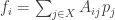
I’ve been talking about Bayesian updating as a discrete-time process: something that happens once each generation for our population. That’s fine and dandy, definitely worth studying, but Marc’s paper focuses on a continuous-time version called the ‘replicator equation’. It goes like this. Let 


where 


Then a little calculus gives the replicator equation:
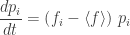
where

is the mean fitness of the organisms. So, the fraction of organisms of the
Note that all this works not just when each fitness
But what does all this have to do with information?
Marc’s paper has a lot to say about this! But just to give you a taste, here’s a simple fact involving relative entropy, which was first discovered by Ethan Atkin. Suppose evolution as described by the replicator equation brings the whole list of probabilities 

Remember what I told you about relative entropy. In Bayesian inference, the entropy
So, in simple rough terms: as it approaches a stable equilibrium, the amount of information a species has left to learn keeps dropping, and goes to zero!
I won’t fill in the precise details, because I bet you’re tired already. You can find them in Section 3.5, which is called “Kullback-Leibler Divergence is a Lyapunov function for the Replicator Dynamic”. If you know all the buzzwords here, you’ll be in buzzword heaven now. ‘Kullback-Leibler divergence’ is just another term for relative entropy. ‘Lyapunov function’ means that it keeps dropping and goes to zero. And the ‘replicator dynamic’ is the replicator equation I described above.
Perhaps next time I’ll say more about this stuff. For now, I just hope you see why it makes me so happy.
First, it uses information geometry to make precise the sense in which evolution is a process of acquiring information. That’s very cool. We’re looking at a simplified model—the replicator equation—but doubtless this is just the beginning of a very long story that keeps getting deeper as we move to less simplified models.
Second, if you read my summary of Chris Canning’s talks on evolutionary game theory, you’ll see everything I just said meshes nicely with that. He was taking the fitness
where the payoff matrix 

Third, this particularly nice special case happens to be the rate equation for a certain stochastic Petri net. So, we’ve succeeded in connecting the ‘diagram theory’ discussion to the ‘information geometry’ discussion! This has all sort of implications, which will take quite a while to explore.
As the saying goes, in mathematics:
Everything sufficiently beautiful is connected to all other beautiful things.


Indeed sufficiently beautiful… Thanks a lot for sorting out such treasures…
The link to Marc’s paper gives an empty arxiv page. I managed to guess this URL to the PDF v1, where Section 3.4 (not 3.5) is titled “Kullback-Liebler Divergence is a Lyapunov function for the Replicator Dynamic”.
Thanks, Flori. Yes, it’s section 3.4. But my link seems to work: it takes me to the abstract page for Harper’s paper; then you can click “PDF” to get the latest PDF.
(I prefer to link to abstract pages on the journal rather than the PDF’s, because it gives you more options: the PDF gives a specific version but there may eventually be a more recent version, or you may want Postscript, or there may be blog links, etc.)
I’m excited because the story I just told seems to be only the beginning of a much larger story: it can be extended in many different ways. Blake mentioned that we can introduce spatial variation. I’m also very interested to see what happens in more complicated models where instead of settling down to an equilibrium, our organisms do what organisms often do, which is keep getting more complex. Someday I want to look at the simplest models that display that behavior. Harper writes (translating to my choice of variable names):
One cause of the complexity might be one of the fundamental tenets of James Lovelock’s Gaia theory, namely that large parts of what a species is “optimising against” is either other species directly (predation, prey, competition for resources, etc) or other species indirect effects (eg, plants altering atmospheric composition). Of course there are some things, such as diurnal cycles, which are to all intents and purposes unchanging no matter what other species do.
Part of the reason for complexity is that when circumstances against which fitness is “measured” change a species tends to evolve Heath-Robinsion-ish modifications to whatever structures are already present, rather than evolve “new, simple” solutions from scratch.
I managed to write the above without making the point explicit: if one evolving species’ fitness depends on some effect of another species which is also evolving, it’s not as if there’s an unchanging fitness “surface” for any one species to optimise against. That, AIUI, is one of the tenets of the Gaia hypothesis.
David wrote:
Yes, this is very interesting to me. It’s when we have a competition between and within species that information theory becomes especially exciting. Why? Because then we have ‘information battles’, where each side is trying to extract information from the other while sending out misleading disinformation. We see this in the way our immune system and bacteria fight each other, or the way insects mimic twigs or more poisonous insects to avoid predation, or the way flowers sometimes trick bees into trying to mate with them, or the way red deer engage in ritual combat that demonstrates their fitness without actually injuring each other.
One thing worth noting is that the replicator equation I wrote down is able to model some of these effects in a simplified form, because the set of ‘types’ can represent ‘strategies’ as well as genotypes, and the fitness
  of the
  th strategy is not just a fixed number, but can depend on the fraction of organisms pursuing each different strategy.
However, the ‘technical conditions’ in the theorem I mentioned—the theorem that says relative entropy decreases as we approach a stable equilibrium—eliminate some very interesting and important cases of the replicator equation. Moral: always read the fine print! And of course the assumption that there exists a stable equilibrium eliminates even more interesting phenomena! Despite the vast amount of attention that’s been lavished on them, stable equilibria are about the least interesting thing to study in any dynamical system. The one true stable equilibrium, if it exists, will be the heat death of the entire universe, when everything dies and nothing interesting happens ever again.
I would have discussed all this in more detail, but I decided the article was getting too long.
By the way, I always enjoy the spirit of scientific caution, so I find it delightful but also sort of amusing how you emphasized the words might and parts: the two words that tend to tone down your claim! It’s amusing, because it’s the opposite of the crackpot who capitalizes key words to emphasize how SURE it is that he’s RIGHT.
(And it’s almost always a ‘he’, just like those deer.)
Applying some free-association in order to connect as many beautiful things as possible, your talk of information battles reminds of the field of cryptography, which concerns itself with the winner of simple types of information battles. For example, public key cryptography gives a practical strategy in the game of ‘send a message to someone else whom you can passively observe while not allowing an adversary to figure out your message’. Then again, there is a simple reason why no animal as far as I know (except humans) use any form of cryptography: The method of communication while there ensuring there is no other individual of the same species in listening range is good enough.
But isn’t every language essentially “encrypted” by default? A language is something that only the community that creates it can use, right? That means every species is essentially as barred from knowing what others are signaling to each other as people or academic disciplines using different languages are, like almost entirely.
To me that has always implied that species are largely fending for themselves, and seeing the world in their own terms. For that problem success would rely on using active learning, in terms of their own language, as the way to discover food and shelter where it’s both plentiful and safe gather.
When you have an active learning task in mind when watching how both the simplest to most complex animals behave it seems that’s exactly what all that “foraging and dodging” animals do is about. Everyone is constantly “sniffing around” with whatever sense organ works for them, taking care of themselves by a least cost strategy. Aren’t the animals who come into conflict with those of other species evidently not being successful at staying out of conflict, like the majority of their population are?
I recall that Cosma Shalizi has some remarks about Bayesian inference as an evolutionary search algorithm.
Thanks! This is the most relevant part, since it describes him having the same sort of epiphany Chris Lee had:
Brilliant. I am an economist. As you say biology is messy, economy is messier. We still do not know much about the real causes of differences in wealth of nations or in wealth of individuals for that matter. What I find is a fascinating (but not proved) analogy. Sometime ago (in 1962) Kenneth Arrow and his friends observed that the productivity differentials between Japan and US are lower in capital intensive (when K/L is very big, like petro-chemicals or telecommunications) and are higher in labor intensive economic activities. Now take any X process as a genotype of ‘doing’ things, if X(i) has a better fitness than X(j) people change the way they do things. My conjecture is that as (K/L) approaches to an optimal stable equilibrium then relative entropy approaches to zero, so the productivity differentials become nil. The similar reasoning applies to labor intensive processes as well, but here the ‘distance’ to the frontier is huge compared to the much more ‘physical’ (high K/L process) system.
Let me give an example, on average people in Turkey can make computers as productive as they make in US (very soon) but on average we will be lagging in terms of making science.
Well at least we may know some stuff about what causes this lag thanks to these kinds of blogs and papers :) and maybe do something about it.
Alper
Hi! I’m not sure I understand your conjecture.
I think I understand this. 1962 was a long time ago, as far as the Japan-US situation is concerned. What’s it like now?
This is the part I don’t understand. You’re saying that when the ratio of capital to labor (that is, K/L) in some industry approaches an optimal stable equilibrium, then productivity differentials between countries approach zero?
(I don’t know what relative entropy you’re talking about here.)
This seems to be an example of something simpler. Here it seems you’re saying that productivity differentials between Turkey and the US are approaching zero faster in industries where K/L is big.
Are there examples of poor countries with very clever people, that are slow at becoming productive in high K/L industries, but quick at becoming productive in low K/L industries?
For example, perhaps the outsourcing of call centers to India? Isn’t that a low K/L industry? CBS News writes:
I mighte have been more precise. The picture about industry-level productivity differentials can be found. at http://www.oecd.org/dataoecd/25/5/1825838.pdf
(Table 2). Notice that both Japan and Germany still lagged US in detergent and food. Let me clarify my point on high (K/L) and lower potential entropy. Assume a continuum of a commodity-service, C(i), as an attribute of how physical (K/L) or how biological (L/K) is the making of that commodity or service. As a very general suggestion I say that as the physicality of the commodity increases, the evolutionary process of finding the global optima becomes faster and faster (or say the distance from the actual best practice that is being spread and the frontier of optimal best practice decreases). That is my point of declining entropy (sort of shrinkage of search space). If I may link the entropy with information (as any untried set of technological-organizational mix) then what I argue is that that information set is larger if the commodity is more biological.
About Indians doing smart things I have no objection. The problem is how general can that be. Let me try to explain. Let assume that US economy produces zillion commodities that can be classified broadly in three groups. X: physical (high K/L), Y: biological (high L/K), and Z: any mix of the former two. India on the other hand can produce only subset of (X,Y,Z). (1) In that subset if the weights of Y goods are high then India’s productivity lag is greater, (2) If the weight of X is small, we reach to same conclusion as we get the weighted average of all commodities. (3) India’s subset of Z commodities will be smaller as probably her X and Y subsets are smaller than US. And as Z set becomes smaller (sort of missing middle) the efficiency gains in Y becomes smaller as the learning space is smaller. If you are good at producing detergent, you will be good at producing soap as well. Can India beat US by just focusing Y goods (like software)? My answer would be no. It has to produce X and Z goods too. As in Turkey if we devote our all resources (money and brain) on science maybe we can get close to US, but then we need cars and detergent as well. In cars we have come a long way and now we are very productive and we export them to Europe. Car is an X good. But it will take longer to be as productive in detergents/food processing and more importantly it will take longer to cover the whole spectrum of Z goods/services that US has.
Do I make sense?
I believe that the interesting research is in the productivity variability between individual workers. Humans are distinct enough in their skills that diversity is highly visible at that level. Check out the superstatistics study of Japanese labor productivity from Kyoto University. They just released a new paper in April (PDF). The trends are highly dispersive over the labor populations, and this latest paper started looking at European labor statistics and they see the same general features.
Thanks for the link. I agree. The interesting part is that for my understanding as an economist there are two components of individual productivity observed ex post. (1) the genuine individual productivity (i) and (2) the extra productivity shock due to the benefits of a public goods (within the continuum of Prisoners’ Dilemma to Volunteers’ Dilemma, as in the comment of Blake Stacey below). I suspect that even if the individual productivities of two groups are same in terms (average, standard deviation) ex ante, the ex post individual productivities will differ in the two different firms with two different (K/L) ratios while doing exacty the same thing, ie. producing cars.
I think the differences between the labor pools lies in the ratio distribution for productivity (Output/Time) accounted for by the different learning curves that pools of workers may experience. Placing a stronger asymptote on the learning curve narrows the productivity disparity (PDF power laws closer to -3) while linearizing the learning curve leads to the -2.
Alper & Web, But if the core problem with labor productivity, is that the aggregate productivity of labor in using the earth is already too high to be sustained, how does further increasing productivity help?? Productivity never created any resources, you know, just increasing access to and higher profits for, depleting fixed resources.
I think that’s the problem with this multi-dimensional problem we face. Most problem definitions are way out of date. For example, the peak sustainable level of CO2 pollution was crossed somewhere around 1960 I think. Every single economic investment relying on the use of fossil fuels since then… should have been assigned an overshoot penalty, like a profits tax for unsustainable development.
It’s a very real redevelopment cost directly caused by pushing economic growth that then has to be replaced with another kind. Today’s sustainability community is itself relatively innumerate, and essentially still wandering around aimlessly not knowing how to calculate opportunity costs like that, though.
So maybe we could frame the calculation, say for the opportunity cost of increasing productivity for resource use… We could just put in any ranges of the variables to just see how to build the equation. Then we’d pass it on to some economists and ask why not treat the economy as a physical system, and have business pay for their consequences?
The basic principle would be that every year the economy is building infrastructure it’ll have to throw away and replace with something else that is sustainable. The question is how present choices can pay for themselves, as a new definition of sustainability.
Phil, As far as labor productivity is concerned, I am just trying to verify the model. This becomes a characterization exercise from an econophysics perspective, and I don’t want to get too far ahead of myself in saying productivity is good or bad. At first it is enough to describe what is happening with the help of a model.
Phil,
It is about what you do with productivity and resulting value/(profits + wages + rents). (1) you can keep on consuming greater and greater amounts of commodities. That will be the end of nature (including the human-beings) or (2) you can free up time/labor time (and consume less; meaning investing in less private goods but more on public goods). If we happen to choose (2) that would also help for sustainability. The point is more political than economic. However, in order be able to do (2) we have to learn and somehow apply the dynamics of increasing individual/team productivities. The advanced countries have to sacrifice much more for the fact that their states and corporations were deriving the capitalist/productivist logic very close to the cliff. The immediate way towards the solution would be redistributing half of the wealth concentrated at the 1 % of households in the world to the bottom 40% in exchange for a commitment to consume and work say 10% less.
Web & Alper, I’d agree with you both,… so long as we’re directing our attention to the behavior of the economic system as a whole. So, as far as we’re not, the cases would be local rather than general.
The necessary approach I come to is to work a little backward in how one defines ‘productivity’. I use the general business definition of more revenue for less expense, to make it a universal definition, and judging any particular for the effect on the whole input/output balance sheet.
I found a way to define those things quite precisely for the productivity of energy use in the world economy. The world’s energy productivity becomes the amount of GDP the world economy produces from a unit of energy. The amazing thing is that that the correlation has been miraculously smooth and steady for the past 40 years, like a simple equation.
For each unit of energy use reduction in producing GDP, the world economy created 2.5 new energy uses, so a “rebound effect” of 2.5. It takes a while for it to make sense, but seems to when you consider that improving productivity makes resource use more profitable. A drive for profits is what causes us to choose those particular efficiencies that release the most added production… thus the rebound effect that contradicts the recent fad that began in the mid 80’s of believing efficiency is a way to reduce energy use. What that community fails to do is separate efficiency from productivity.
The net effect is the world commodities bubble. Our drive for productivity creates persistently escalating resource demand, which is now meeting the leading edges of “peak everything”, as we’ve all been talking about. The fact that we’re trying to create ever more resource demand to solve the problem of having too much resource demand… is one of the key problems I’m trying to figure out how to communicate. Virtually everyone seems so firmly committed to both at once, that considering the contradiction seems off the table.
For references see: “Why efficiency multiplies consumption” – synapse9.com/pub/EffMultiplies.htm
“A defining moment for Investing in Sustainability” – http://www.synapse9.com/pub/ASustInvestMoment-PH.pdf
Web, to clarify my concept, since we don’t have different words for different kinds of productivity yet, I use it to mean everything that enables production. As I look around what I find is the “magic” of every productive innovation is allowing a new kind of organization of the parts of the business system that it effects. The example is “drip irrigation” that allows the development of semi-arid landscape that was useless before. I think being inclusive that way is needed. Would you agree?
Alper,
Your solution is a variation on the one that JM Keynes proposed, in Chapter 16 of his big book. His method is shocking to money people enough, be sure, but would not need so much politics. He focuses on profitability, and how accumulating investment savings as it “wrecks the earth” becomes unprofitable….
To maintain the profitability of the economy as a whole, there is a necessity for those with investment earnings they might otherwise add to their savings, to instead divest them as gifts or spending for good works of some sort. I’ve written a good bit on that, though I haven’t written papers on it for over 20 years, for complete lack of anyone to see the need to discuss how to do it…!
What I’ve written recently is in blog posts, Google search [site:synapse9.com/blog/ keynes] and browse my “Natural Economy” category [http://synapse9.com/blog/category/natural-economy/] fyi
An extra wrinkle probably worth considering is, “What happens when a bug can only interact with its geographical neighbours, so fitness is defined as a function of local population densities instead of global ones?” For example, when the players in an evolutionary game are arranged on a graph, the topology of the graph turns out to have a strong effect on what kinds of equilibria can exist. A decent, recent-ish review on this topic is Szabo and Fath (2007), “Evolutionary games on graphs” Physics Reports 446 (4-6): 97-216, arXiv:cond-mat/0607344.
Another possible avenue to explore is, “What happens if the effect on bug of the individuals it meets in its life is not a linear function of the genotypes of those organisms?” Recent work I know of which looked at this includes the following:
M. Archetti and I. Scheuring (2011). “Coexistence of cooperation and defection in public goods games” Evolution 65, 4: 1140-48.
J. A. Damore and J. Gore (2011). “Understanding microbial cooperation“. Journal of Theoretical Biology DOI:10.1016/j.jtbi.2011.03.008.
Blake wrote:
Yes! Marc Harper is actually thinking about this. You’ll note I keep seeming to ignore your suggestion to add space to the game, for example in my discussion of stochastic Petri nets, where you’re doubtless eager for me to put my bugs on a lattice and start thinking about reaction-diffusion equations. I definitely want to do this, but I’m so busy learning about other issues (like the connection between stochastic Petri nets and information geometry, hinted at here) that I’ve been putting off introducing space.
One excuse for this is that it’s easy to do: I can take my set of ‘genotypes’ and formally declare that I’m reinterpreting it as a set of ‘genotypes at particular locations’, e.g.
  where
where  is a set of genotypes and
  is the set of vertices of some graph. So we won’t have to undo the basic formalism; we’ll just have to think about it in a new way. And of course the fun starts when we investigate the new questions that arise.
Thanks for the references on more nonlinear versions, too!
Take your time! I’ve been enjoying the series so much that I don’t want to force your hand. If you only wrote about the stuff I’m currently thinking about, I’d never learn anything new! :-)
Altogether too many science discussions I’ve seen of late have been real downers. Either their subject matter tends to severe doom-and-gloom-ism, or the loudest people involved in them persist in missing the point about what other people are saying. So, it’s very good indeed to have a conversation going on where I can think, “Yep, science is fun!”
On a more technical note, there are a couple different sorts of nonlinearity one should be aware of in this context (represented, more or less, by Archetti–Scheuring and Damore–Gore respectively). Suppose that we’re trying to figure out the fitness of the individual, call it
  , as a function of the genotypes of the organisms with which it interacts,
  . To start with, we might as well assume that the total effect of multiple causes taken together is the sum of the effects those causes would have taken independently, and that the size of the effect grows evenly with the size of the cause. So, we write a linear equation,
where we’ve written the parameters with a as an homage to the “regression coefficient” jargon common to the art. The idea is that if we had a whole bunch of measurements from a laboratory or a field station, we could run a regression analysis and figure out what the values of these coefficients should be. Of course, we can feed any set of numbers we want into the our statistical software package; saying that the results have any predictive value is a stronger statement, which requires making a claim about the linearity of the interactions at work.
You can find people who prefer to consider genotype or trait values relative to the social circle to which the individual belongs. This is like what we physicists do when transforming from the laboratory frame to the centre-of-mass-frame, except it’s a “centre-of-social-circle” frame. This coordinate change means that the parameters
  get mixed up with each other, but since the equations for the next step of the computations — figuring out how the genetic composition of the population changes as a result of these fitness assignments — are also linear, everything works out pretty simply.
We can make the relationship between genotype and fitness more complicated in lots of ways. We could wrap a nonlinear function around the whole sum, for example. This is the kind of nonlinearity that Damore and Gore are mostly talking about, I think. We could also make a multiplicative combination of genotypes.
A parable: several of my friends have recently been or will soon be moving to new apartments. (In the Greater MIT Metropolitan Area, nomad academics are doing this all the time.) Three of them, called here 1, 2 and 3 to protect the innocent, have to move a heavy object, like a piano or a drill press left in the living room. Hefting the piano requires investing a certain amount of harrumph, and they can only move the piano if all three heft simultaneously. The payoff to flatmate is, using
  to denote “doing nothing” and
  to indicate “hefting the piano”,
The cost and benefit
  parameterize the situation, which Archetti and Scheuring call a Volunteer’s Dilemma game.
Blake wrote:
Okay, I’ll take my time before bringing in space. Maybe it’s some weird counter-reaction to working so much on gauge theory, quantum gravity and the like, but it’s sort of fun to forget about space for a while, and focus on my current obsessions: information, probability, and networked systems.
(Hmm, but my old obsession in quantum gravity was trying to ‘dissolve’ our old notion of spacetime as a manifold and treat it as a kind of networked quantum system, namely a spin foam. So maybe we don’t really change that much.)
Some of the subject matter of this blog could easily lead to severe doom-and-gloom-ism, but I have trouble staying depressed. At first when I quit my old work and decided to tackle environmental issues it took a conscious decision not to become depressed. I decided the right attitude was that expressed by Gimli in the movie version of The Lord of the Rings:
Tolkien himself would never write such a disgustingly Hollywood-esque line, but as a rallying cry to tackle a monstrously difficult problem it’s not bad.
More recently, I find it hard to avoid relapsing into the enjoyment of understanding for its own sake. I guess it’s part of a balanced diet.
Despite the post-apocalyptic black look of your blog, a design choice I’ve never fully understood (though I finally found out what ‘after sunclipse’ means, and discovered it wasn’t the end of the world), you always seem to have fun thinking about ideas.
(By the way, why did you close comments on your article about logic puzzles so soon? Were you afraid of an onslaught of outraged logicians, or is it because you’re ‘upgrading’? I want to leave a comment!)
I switched off comments on my blog because I really wasn’t using the site enough to warrant dealing with spam getting through the filters — just a way to give myself a little less to fret about each day. Now that I’ve upgraded the software and actually posted something again, I should look into the configuration options and see if I can find some commenting scheme I like.
Okay, then for now I’ll have to comment on your blog over here on mine: you can outsource the spam filtering to me.
WordPress has a really good spam filter, by the way. Almost no spam gets through. Occasionally comments with lots of links get mistakenly identified with spam. But spam is really not something I worry about.
Anyway, it’s quite off-topic here, but when you said
I had to cringe, because while The Hobbit is a great children’s book, it was definitely written for children, while The Lord of the Rings is very deep and interesting, especially for anyone who enjoys languages or mythology. I’ve read it about 5 times, twice out loud with my wife. If you can’t abide fantasy of any sort then you’re excused, but really Tolkien has done an amazing thing, which is to pick up a tradition of myth-making which faltered sometime around Beowulf and breathe new life into it.
The first chapter is somewhat in the style of The Hobbit, but it gets deeper quite quick.
I believe that I have a method to extend the general idea to finite populations with spatial structure, e.g. occupying vertices on a graph, which is unpublished. For a finite population birth-death dynamic like the Moran process, you can look at the expected KL-divergence (the expectation is taken with respect to the transition probabilities of the process), which now plays a role similar to a Lyapunov function, but for a probablistic dynamic rather than a deterministic one. It is minimal at the rest point, decreasing toward it, etc, and is not too hard to work out in some common cases for two player games linear games.
You can take the same approach with a population replicating on a graph — it is a process with many more states and possible transitions, since the key variable is no longer just the cardinality of one of the types of players. Rather it is a graph coloring that can change one vertex at a time and in principle the computation is quite similar. Unfortunately it is also combinatorially unwieldy for arbitrary graphs.
Others have taken different approaches. The graph structure can be used to develop a continuous replicator equation approximating the behavior of the population on a large graph, using the adjacency matrix of the graph to modify the fitness landscape. If I recall correctly, in some cases these results are exact in large population limits, but this tends to hold analytically (as far as I know) only for graphs with very regular local structure, such as k-regular graphs.
Sounds fascinating! I look forward to reading more when the “finite populations with spatial structure” part gets published.
Look up Relative Abundance Distribution to explain quantitative species diversity.
The typical RAD distribution follows closely the Zipf-Mandelbrot power law, which is easily derived by applying a maximum entropy dispersion on rates of evolution and threshold levels. It is so simple as not to be very interesting apparently. Is it ever interesting when you apply randomness and disorder to rates and get exactly what we empirically observe?
The Wikipedia article is short, tantalizing, and uninformative. When I tried to get something more useful, I found this article of yours:
• WebHubbleTelescope, Dispersion, diversity, and resilience, The Oil Drum, 27 February 2010.
It’s interesting, but it will take me a while to understand it! I’ll need to start by pondering the Zipf-Mandelbrot law, which says (for example) that the number of organisms in the th most abundant species is proportional to
for some values of and
and  . Are you trying to tell me that this distribution maximizes entropy subject to some constraints? I’m pretty ignorant here.
It’s unfortunate that most of the commenters on the The Oil Drum article didn’t dare ask you questions about what you meant, instead resorting to remarks like “there are few things in life which depress me as much as modern man’s superimposition of his mentally-fabricated order upon a Natural world which we know so little about”.
And it’s particularly unfortunate (or funny) that some commenters complained you were using too much math, given how much more math is used in the Nature article you were discussing:
• Igor Volkov, Jayanth R. Banavar, Stephen P. Hubbell, and Amos Maritan, Patterns of relative species abundance in rainforests and coral reefs, Nature 450 (2007), 45-49.
John,
I think of RAD as a race among closely related species to achieve a specific adaptation level that will allow them to achieve relative dominance (i.e. population density). This is what I tried to derive in The Oil Drum article. That site doesn’t have any equation markup facilities so I spelled it out as clearly as I could.
A very short-hand way to think about the idea is that we have two random variables that describe an adaptation. One is the abstract adaptation level the species needs to achieve , and the other is the time it takes to reach that level
  . Let
. Let  . The math problem is to find the PDF of
  if
if  and
and  are independent and both maximum entropy exponentially distributed with some mean.
This turns into the basic ratio distribution derivation,
where is the median value for adaptation rate. Note that the distribution has no mean value.
This result matches the Zipf-Mandelbrot law with a value of for the PDF. This is the exponent most frequently observed as well.
So I believe what we are observing in nature is a continual race to achieve dominance based on the rate of advance of various species. When certain ecological regions are more isolated (local) the agreement is better, and when the region goes metacommunity, then the distribution becomes broader as different starting times get merged. This essentially says that species can have different time spans in which to adapt, instead of adapting together in the case of a localized region. The metacommunity distribution differs from the Zipf-Mandelbrot but it is still very easy to derive.
So that is the basic model but I am not sure any of the ecologists or evolutionary biologists are assuming anything this elementary. I like it because it parsimoniously explains much of what we observe in nature. An explanation more involved may be more realistic but it won’t necessarily match the empirical data any better.
BTW, I agree with your assessments on the commentary on various sites. Your site is different, top-notch when it comes to signal/noise ratio. Part of the problem is that we will always run into commenters who are sincere but cynical as to how much any of this mathematical analysis will help in the greater scheme of things.
If the replicator equation is a continuous-time version of Bayesian conditionalization, does that allow for a more dynamic interpretation of movement in the space of probabilities? I can’t remember where just now, but you were wondering somewhere why I keep mentioning Amari’s ideas of inference as movement along a geodesic.
I can’t wait to have a look at this material when I have a moment. Some Bayesians are moving away from seeing conditionalization as the main updating mechanisms in the direction of maximizing or minimizing relative entropy, the idea being that it’s rare that you learn only new data.
In fact you can see conditionalization as a special case of maximum relative entropy. Caticha and Griffin describe how this works in the case of learning data and moments of a target distribution in this paper. Maybe there’s a continuous-time version.
But there’s also the minimum relative entropy principle. I’m not sure I ever squared these two principles with each other.
David wrote:
Right, exactly!
If you read that long quote from Cosma Shalizi in my reply to Nathan Urban, you’ll see he thinks of Bayes’ law as a special case of a discrete-time version of the replicator equation. This is basically the same realization Chris Lee had.
But turning this on its head, this means that a special case of usual continuous-time replicator equation can be seen as a continuous-time version of Bayesian updating. Elsewhere in his article Shalizi explains this further:
By ‘natural example’ he must mean an example from Bayesian learning: the truly natural example shows up in biological evolution!
Right. I’ve been thinking about you a lot in the last few days! If you’d told me earlier that Amari’s ideas were the key to understanding biological evolution as a learning process, I wouldn’t have been doubting their usefulness. But you did more than your share just by making sure I was mentally prepared for what Marc Harper had to say!
Hmm. In our conversation, he did mention Amari’s work on geodesics and those ‘dual connections’. These aren’t mentioned in his paper, so I’m not sure there are cases of the replicator equation where it’s following a geodesic. (That would be good to understand.) But you’ll see that Harper’s paper has a lot to say about the Fisher information metric. You’ll like his paper, I’m sure.
I’ve collected everything I know about entropy minimization and entropy maximization here. Like you, I’m confused. You’ll see some very interesting comments by David Lyon and Tomate. But I still haven’t had time to think hard about this subject!
A good paper of Fujiwara and Amari for gradient systems, dual connections and their geodesics, and several explicitly worked examples is:
A. Fujiwara, S. Amari, Gradient Systems in View of Information Geometry, Physica D, Vol.80, pp. 317-327, 1995.
In particular, section 5.4 discusses the replicator equation and how it is the gradient for symmetric linear fitness landscapes, and that the mean fitness is a potential function. This is not always the case for the replicator equation, which is fortunate or unfortunate depending on your perspective.
There are also other interesting examples of the dual manifold structure including maximum likelihood estimation, the EM-algorithm, linear programming.
I see in Marc’s The Replicator Equation as an Inference Dynamic the idea of iteration of Bayesian conditionalization as evidence comes in. Given that the fitness of a hypothesis is given by
  at step
  , we see that the fitness function varies with time. Do people study the replicator equation, discrete or continuous, with a time-dependent fitness function?
As a side note, my colleague Teddy Seidenfeld showed back in the 1970s that updating by conditioning is not a special case of updating by extremizing relative entropy. See Seidenfeld 1979 and (even more explicitly) Seidenfeld 1987. To the extent that one trusts the decision-theoretic, these-are-the-axioms-of-rationality justification for Bayesianism, one should of course update by conditioning.
I’ll have to have a look again at the Seidenfeld papers when I have the chance. Have you seen Harremoes’ work (mentioned here) on conditioning as projection to closest point on a submanifold?
Some of the proposed problems raised for the relation between conditioning and minimum relative entropy are resolved with precision about which space of events is being considered, as in Giffin and Caticha’s paper. The space of models for the bias of a die and the space of outcomes of a series of a throw have to be treated separately.
I have not read Harremoes’s paper. I have read Giffin and Caticha, and IMHO it doesn’t deal with the type of issue Seidenfeld raises at all.
The space of models for the bias of a die and the space of outcomes of a series of a throw have to be treated separately.
Indeed. We might call these the “parameter space” or “hypothesis space”, and the “sample space” respectively — just like actual statisticians have done since time out of mind.
Just a quick note to mention the recent “novel perspectives on MaxEnt” special issue of the ecology journal Oikos.
Talking about a heated debate, the argument between mechanism and resorting to statistics in explaining diversity has centered around the use of MaxEnt. This is essentially a battle between ideology (mechanism implies that there are biological and behavioral reasons for diversity) and pragmatism (the use of approaches such as MaxEnt). Many of the idealists of course want to discover new mechanisms to explain relative abundances but the pragmatic approach has worked too well to match the distributions observed.
The Oikos link and Steven Frank’s work further fuels the debate.
I’m pleased and flattered that actual physicists have noticed my little post at Oikos (and haven’t (yet?) exposed my brief remarks as complete nonsense!)
I think Web Hub Tel has correctly summarized the debate in ecology to this point, but I think the debate is resolving itself. I think ecologists are increasingly realizing that many of the common ‘macroscopic’ patterns in which they’re interested can be generated by a wide range of different ‘microscopic’ mechanisms. So there’s little hope of being able to ‘read off’ the underlying mechanisms just from looking at the patterns (a lesson ecologists seem to need to relearn once a generation or so). What Steven Frank’s work highlights, at least for me, is that we still don’t *really* understand why it is that certain patterns tend to emerge from many different combinations of underlying mechanisms.
I’d be very interested to hear any comments anyone on this blog cares to offer about Frank’s work, especially the stuff linking commonly-observed patterns to their natural measurement scales. I feel like I’m comfortable with the stuff linking Fisher information to natural selection, which is well articulated on this post as well. But the measurement scales stuff is something I’m still struggling a bit with. I’m not clear if it’s a deep insight, or merely replacing one thing we don’t understand with another (replacing ‘Where does the pattern come from?’ with ‘Where does the natural measurement scale come from?’)
Jeremy: regarding patterns, what is the recent status of studying self-similarity in diversity? For example:
• J. Harte, Self-Similarity in the distribution and abundance of species, Science 284 5412 (9 April 1999), 334-336.
Has this been subsumed by Frank’s work?
Nice to have a real expert in the field participating here!
oikosjeremy wrote:
In the physics trade, this is known as “universality” — a fairly grandiose name for the idea that systems which look different at the micro-scale can have the same behaviour at the macro-scale. A set of such basically-equivalent systems is known as a “universality class”, and the different universality classes we know about have names, usually chosen for the prototypical example of the class: two-dimensional Ising, (2+1)-dimensional directed percolation, Kardar-Parisi-Zhang surface growth, and so forth and so on.
Unfortunately, the situations where we know the most about what universality classes can exist and how they are related — where we have built a “Periodic Table” of universality classes, so to speak — are pretty far removed from ecology. (Or so it seems to me.) We know that the critical points of two-dimensional statistical-mechanical systems in thermal equilibrium can be organised through the ADE classification of conformal field theories, which relates in deep ways to weirdnesses all throughout mathematics, but I’m not sure how much that helps anyone trying to understand a bacterial biofilm, let alone a rainforest!
There is a statistical-physics textbook which talks about universality in a not-too-forbidding way, and explains how it relates to scale invariance: Sethna’s Statistical Mechanics: Entropy, Order Parameters, and Complexity (2006). It’s intended for people who want to apply the ideas born in statistical physics to subjects outside the boundaries of that topic, narrowly considered. Best of all, a PDF version is free online. Chapter 12 is the relevant one.
In reply to Web Hub Tel (below; that comment doesn’t seem have a reply button):
IIRC, Harte’s 1999 self-similarity paper turns out to have some problems (I recall a nice paper in American Naturalist pointing this out). It’s my impression that self-similarity turned out to be a bit of a dead end, as Harte himself has lately been pursuing MaxEnt approaches instead.
With regard to Frank, although MaxEnt has been very widely discussed in ecology in the last few years, Frank’s own work seems not to have been much noticed by ecologists, presumably in part because Frank’s been publishing in evolution journals. The main goal of my post over at the Oikos journal blog was to call the attention of ecologists to Frank’s work.
In reply to Blake Stacey:
So, when are you physicists going to get around to completely figuring out universality? ‘Cause it would really be useful to us ecologists if you could do so! We ecologists are standing her with our arms crossed, tapping our feet and waiting on you! ;-)
Blake, Applying universality is kind of over-kill for most of the mundane empirical observations made, isn’t it?
All these PDF’s that have power-laws close to -2 (like species abundance) are likely just examples of ratio distributions or other algebras of random variables. They have little to do with new collective phenomena of matter and more to do with the amount of garden-variety disorder that exists in natural systems. Some people refer to this as superstatistics.
This is exactly what Jeremy is saying by “common ‘macroscopic’ patterns in which they’re interested can be generated by a wide range of different ‘microscopic’ mechanisms.”
The microscopic mechanisms may not have to be that different; they could also operate under varying local environmental conditions which change the rates and times for behaviors.
So we jump through all these hoops trying to find a complicated mechanistic explanation when a simpler one, with disorder sprinkled over it, will suffice.
In other words, what happens when we go down the rabbit-hole and find nothing revolutionary there? I don’t mind, because I just want to explain pragmatic stuff like oil depletion and climate change. And I think the ecologists have the same pragmatic goal in how to understand diversity and perhaps protect it from completely disappearing before we end up completely fouling our environment.
I still find the math interesting, because I run into these brain-teasing conundrums all the time, and the principle of maximum entropy is a useful tool for situations when you have little additional knowledge of the statistics of the disorder.
I tend to think of “universality” in a broad sense of the term, according to which, e.g., the Gaussian distribution arising from the central limit theorem is an example of universality. (See ex. 12.10 and 12.11 in Sethna’s book for a higher-falutin’, renormalization-group based justification of this.) I would agree that the elaborate mathematical machinery built up to understand universality in the kinds of systems statistical physics care about is probably overkill (or just inapplicable) here.
(I bought Sethna’s book a couple of years ago and now find that it’s a free PDF, oh well he got some royalties out of me :) It is a beautifully laid out book BTW.)
The Gaussian is one of three stable central limit distributions. The others are the Levy and the Cauchy (the latter a power-law of -2). Then those must be universal in a similar sense. So for something like the fat-tail Cauchy, if you add up enough random variates from this distribution you still get a Cauchy. In other words, the convolution of a Cauchy with a Cauchy is still a Cauchy — easy to prove via Fourier analysis as well. This also explains the ubiquity of the -2 power-law through many experimental observations, as it shows great stability against perturbations.
I just find it unusual that you don’t find many researchers admitting to how common this distribution is and how easily it can be explained. Didier Sornette wrote a book similar to Sethna’s in scope (Critical Phenomena in Natural Sciences) and he has a Chapter 14 on “Mechanisms of Power Laws”. His simplest example is the change of variable approach which conserves probability.
p(x)dx = p(y)dy
if y = 1/x, then p(y)=p(x)/y^2, which essentially transforms into the same power law.
I think its a simple matter of making observations in reciprocal space, say in rate versus time, that we see many of these distributions. Yet it is very unusual to find literature pointing this out. Even Sornette doesn’t dwell on the simplicity of this reciprocal mechanism, preferring to expound on a lots of other mechanisms centering around criticality. It is almost as if we are searching for something more complicated than a simple mathematical identity, because we want to find something more complicated. Could that be the salient observation?
I like simple identities. If they’re simple enough, even I can make use of them! :-)
(I bought myself a print copy of Sethna’s book a while back, too, after I’d read chunks of the online PDF.)
WebHubTel wrote:
As Blake notes: no, not if you understand ‘universality’ in its fully general sense. In this general sense, ‘universality’ simply refers to any mechanism that leads a wide class of phenomena that differ in their details to act ‘the same’ in some significant quantitative way.
The power laws you like so much should be excellent examples of universality. And this is actually why you like them so much!
The kind of universality that people in statistical mechanics like is the kind where ‘zooming out’ allows you to ignore the microscopic features of some material. As we repeatedly apply some ‘zooming out’ operator, usually called a ‘renormalization group transformation’, we sometimes find that the fine-grained details ‘wash out’ and become irrelevant. We say then that the situation approaches an ‘attractive fixed point’ of the renormalization group, where washing out further fine-grained details doesn’t do anything.
The upshot is that in these situations, the microscopic details don’t matter if you’re only interested in certain questions. What matters is the attractive fixed points.
But this business you mentioned about the Central Limit Theorem is saying that the Gaussian, Cauchy and Levy distributions are also attractive fixed points of a certain transformation! That’s what the theory of stable distribution is about, apparently.
By the way, I’m just saying stuff Blake already said. It’s news to me, and it’s cool, so I feel like repeating it.
I have a feeling that if I try to claim universality by taking the reciprocal of a widely dispersed observable, then quite a few reputable physicists would take issue with my claim. I always thought they reserved this meaning of universality for critical phenomena.
Taking the reciprocal of something and getting something else does not qualify as ‘universality’. But ‘universality’ includes any mechanism that causes a wide class of phenomena that differ in their fine details to act ‘the same’ in some significant quantitative way. There are lots of examples outside the realm of critical phenomena.
An example of this term is used from Schuster and Just’s book Deterministic Chaos:
Noise in its 1/f form is definitely one of those phenomena that is purely garden-variety disorder with a reciprocal origin. The time-domain representation is random telegraph noise that behaves according to a memory-less Markov process. The auto-correlation of this is a two-sided exponential and the Fourier spectrum is a Cauchy, which gives the power-law -2. The 1/f spectrum derives if the Cauchy is integrated over many characteristic median frequencies, which relates to its ubiquity across many different natural sources.
I have written more on this topic in my book, but Milotti has written a really good review. He says in his concluding remarks “My impression is that there is no real mistery (sic) behind 1/f noise, that
there is no real universality and that in most cases the observed 1/f noises have been explained
by beautiful and mostly ad hoc models.”
Milotti, E., “1/f noise: a pedagogical review”, invited talk to E-GLEA-2, Buenos
Aires, Sept. 10-14, 2001, http://www.nslij-genetics.org/wli/1fnoise/milotti02.pdf
Yes, universality turned out to be a big deal in the study of dynamical maps and chaos, starting with the work of Feigenbaum.
From section 8 of Milotti (2002):
which is just what universality is. We identify (or make an informed guess about) which equivalence class a system belongs to, and then we generate predictions about the system by studying a simpler representative of that class. (For example, we draw a density/temperature curve for carbon dioxide near its critical point by calculating the magnetisation/temperature curve for the 3D Ising model, or we study period-doublings in some hairy chaotic map using predictions from the simpler logistic equation.)
This is not to say that identifying a single common feature is enough to declare two systems equivalent!
I forgot to mention: see Sethna’s exercise 12.4 for universality classes in dynamical maps.
If the question is whether
then I don’t think that they do, and more importantly, I don’t think that they should. For example, Henkel and Pleimling’s Nonequilibrium Phase Transitions, Vol. 2 discusses “aging processes”, slow changes of bulk materials under mechanical forces or after abrupt thermal quenches.
(Bold emphasis theirs; I’ve elided a few sentences referring to a figure I can’t reproduce.)
While the most robust and deeply explored examples of universality may belong to statistical physics and its critical phenomena, I can’t see a good reason to restrict the term to that subject.
A point we should clear up is what we mean by “critical point”. If we mean, “That point on a phase diagram where the liquid-gas coexistence curve stops, or its analogue for a magnet”, then universality is definitely a more broad concept. If we mean, “The fixed point of some kind of renormalization-group transform”, then we may well encompass most of the classic examples which go back several decades: liquid-gas transitions with critical opalescence and all that, but also the period-doubling route to chaos, random walks, stable distributions, nonequilibrium percolation phenomena, etc. We may, however, be leaving out examples which are closer to the edge of the unknown, which should by rights be recognized as “universality”, and which indeed have been labelled so.
(My own work has been on nonequilibrium systems which would exhibit universality in other regions of parameter space, but are ruled by idiosyncrasies in the regions where I find them. So, I know first-hand that universality classes aren’t the whole story. In fact, one upshot of this particular project has been to throw cold water on the claim that the system we’re studying will naturally tend to a critical point and thus universality will hold . . . a story I’ll be able to tell in greater detail when it hits the arXiv.)
We also see a related problem called creep failure attributed to elastic and plastic changes early in a deformation process. Sampling from a population of parts undergoing deformation leads to the observation of a bathtub reliability curve. The bathtub curve describes more frequent failures observed early on, leading to a low plateau, followed by an increase in failure rate again for long-lived parts.
I modeled this behavior via MaxEnt principles in The Oil ConunDrum. The fact that a bathtub curve even exists suggests that highly dispersive behaviors play a predominant role in failures. Again, I would ascribe this more to material on-uniformity than to any universality. To be able to separate out other interesting critical phenomena from the inherent disorder has to be a tough job.
I also like the popcorn popping example that I describe in the book. Is a kernel of popcorn popping a critical phenomenon or just a failure in the strength of the highly variable pericarp shell?
The time-dependent probability that an individual, isolated popcorn kernel will pop is, I expect, a consequence of material properties and physical idiosyncrasies peculiar to that kernel. However, if we pop a whole bunch of kernels and gather statistics on the results, the shape of the overall curve may be independent of much of those details. By analogy, if we shake a box of coins and count how many
  land heads up, we expect the histogram of
  over many repeated trials to approach a Gaussian distribution, because
  is the sum of multiple uncorrelated small contributions. We predict a Gaussian curve whether the coins are copper or gold. The only “critical point” here is the one in function space: the Gaussian distribution is an attracting fixed point under an RG transform.
For a failure-rate or survival-time analysis, I’d guess that you might end up dealing with extreme-value statistics, where the universality classes go by Gumbel, Fréchet and Weibull.
The problem is that popcorn popping statistics is not close to Gaussian. The classic experiment I recount is to pop the kernels individually to get rid of any collective effects and it really just obeys Arrhenius rate laws subject to variability in the shell strength and moisture content. If the fall-off was Gaussian it would show up as an inverted parabola on a semi-log scale; yet it yields a straight line reflecting first-order kinetics as the kernels are heating up and exponentially expanding the pressure within the kernel. In other words, without the underlying accelerating kinetics it would be a simple power-law fall off. I don’t think a lot of people understand how these counteracting effects (acceleration and dispersion) hide the real process that underlies the behavior.
I got interested in this because popcorn popping is very similar to the derivation of the logistic via accelerated dispersion for the classic Hubbert peak of oil discovery. What we have here is acceleration in technological prowess combining with a strong dispersion in this acceleration. The result is the classic Logistic sigmoid. No one seems to grok that this can occur, and instead you get the conventional Verhulst deterministic solution if at all.
As far as the extreme value statistics for failure rate statistics, I don’t really believe much of that applies, especially the Weibull, which needs to be split into three different regions to explain the bathtub curve. If you look into it, the bathtub curve is actually very strange, it has huge tails on both ends, almost the exact opposite of what the extreme value statistics is trying to show. In other words, the extreme values are at short times and long times. That is really hard to explain unless you assume a huge dispersion. I don’t want to explain just the tail-off stats, I want to explain the entire curve.
So how do you get universality if you want to explain the entire curve instead of just the tails ala extreme value statistics?
I find it all fascinating stuff and just note the difficulty in disentangling any interesting phenomena that may lay lurking underneath all the maximum entropy disorder.
Not having thought deeply about popcorn before (and your take on it certainly looks reasonable!), I was thinking of a scenario vaguely like the following:
Let’s say we have a population of widgets, and each widget is composed of many parts. If any part of a widget fails, then the whole widget goes bad. So, we’d like to know the probability distribution of the most vulnerable part — the “weakest link” — as a functional of the probability distribution of part vulnerability. If the latter falls exponentially in its tail, then the former will be a Gumbel distribution. (Gaussian distributions for the parts imply a non-Gaussian curve for the whole! The part distribution doesn’t have to be Gaussian, either — it could be asymmetric or what-have-you. We only care about the tail.) Other conditions on the tail of the part-vulnerability function imply other forms for the widget-level vulnerability: a power-law tail yields a Fréchet curve, for example.
The only “universality” here is that the type of curve we see at the widget level depends on a qualitative property of a portion of the part-vulnerability probability distribution. Lots of different “micro” phenomena yield the same type of “macro” curve.
Note that I’ve neglected the possibility of correlations among parts within a widget, as well as time dependence and all sorts of other things. Sufficiently strong correlations among parts would spoil the picture of classic extreme-value theory (this happens and has been studied a lot in, e.g., random matrix theory).
I’m going to check out of this thread now and try to write a “what physicists think about ‘universality'” piece which presents the matter in a more coherent way than I’ve done here.
Blake,
You convinced me that the popcorn popping statistics that I derived is essentially the same as Gumbel type 1 and I can work the cumulative equation down to something like this for large t=time.
exp(-exp(-t))
So that is what I am getting at in that you take a model of what you think the behavior is and then add the dispersion in until you can match the data. The distribution parameters are then reflected back into the parameters of the model.
Now I lost track of what we are discussing. I thought my point is that you have a huge amount of disorder in these processes and you just use simple models of rate and variability to describe the statistical behavior.
It’s fascinating, though my math stopped at tensors and topology, it seems I can understand much of this discussion in terms of the natural phenomena referred to. Things like how John nicely defined universality.
I’m struck though, by how very localized “universality” then becomes. The way natural processes work, every natural system takes place individually, and in a way that makes the local and particular fine grain processes of developmental construction of accumulating sequences of events quite essential to the workings of the whole. That then seems naturally missing from any of the universalities of information theory.
It brings to mind the reason information can’t serve as a basis for reality, that it contains only symbolic energy. Isn’t there still some need then, for a physical world to test one’s information theory against?
Blake wrote:
Great! I was actually thinking of soliciting such piece from you. If you mail it to me, I can run it as a blog entry here.
Phil wrote:
‘Universality’ is not a concept from information theory (though it could be applied there). It’s a concept from physics. You can read about it here.
Physicists mainly focus on fairly simple systems. Suppose for example that we are standing on a sandy riverbank on a windy day, trying to understand what’s going on. Physicists might focus on the flow of water down a channel, or the gradual falling of sand down a sandpile, or the flow of wind over an obstacle — or the way water molecules tends to form temporary clusters as they collide, or the crystal grain structure of silica in a particular grain of sand, or the way air molecules interact as they collide. Even these ‘simple’ systems are so complex that physicists need concepts like universality to extract aspects that can be understood.
Physicists typically don’t take the next step and study how all these pieces interact in an attempt to create a full model of the scene you’re looking at. Why not? The main reason is that it’s extremely hard: it’s a full-time job, and it’s not physics. So, physicists typically leave it to river-bank-ologists (or specialists of whatever relevant sort) to go ahead and put together the pieces needed to understand a specific complex system.
There is a division of labor here.
Yet again you seem to be reminding us of some old news: science uses the experimental method.
Information theory is a branch of applied mathematics that studies quantitative measures of information such as Gibbs-Shannon entropy (for classical systems), von Neumann entropy (for quantum systems), algorithmic information (for data in the form of a specific string of symbols), and many more. You can read about it here.
Insofar as it’s a branch of mathematics, information theory involves proving theorems and the like. Since I’m a mathematician, this is the aspect I’m good at. Again, there’s a division of labor here. These theorems don’t need to be tested against empirical data, though they draw inspiration from empirical concerns, and their usefulness is in part measured by their impact on empirical questions.
But since it’s a branch of applied mathematics, information theory is widely used in communications technology, thermodynamics, natural language processing, cryptography, neurobiology, evolutionary biology, and many, many forms of data analysis. These are pursuits whose success is measured empirically. And the people who engage in them do not usually need to be reminded of that fact. Sometimes they do, but equally often they need to be reminded of the value of pure reasons.
By the way, I’ve been enjoying your recent posts here a lot. It’s only when you try to inform us that science uses the experimental method, and conflate mathematics with science, that I get tetchy like this.
Someone reading this thread would conclude that the most likely biodiversity distribution would be governed by extreme value statistics. After all, life itself is very improbable, and any species has to go through lots of hoops to survive at all, and so we pick from the Gumbel, Fréchet or Weibull extreme value distributions and see if they fit any of the empirical data sets. If they don’t match anywhere to a close fit, you have to start with a different hypothesis which excludes this universality class. Isn’t that part of the scientific method that most grade-schoolers are exposed to, namely hypothesis-then-test?
John,
Thanks for the full reply, and clarifying how you see the difference between physics and information theory, which we might discuss further. I hope you also recognized my intent was to point out some gaps in that “normal division of labor” that, as I see it, cause serious problems for the applicability of the work of various disciplines caused by that separation of tasks. That’s what I really was intending to point to.
It may be popular, but I think rather inaccurate for you to say, that:
There absolutely IS solid and useful universal categorization using the language of physics that applies to what you dismiss as “river-bank-ology”. That’s the problem with your statement. The useful physics is in the sequence of energetic processes necessary to construct local continuities of developmental change.
I’m of course curious why that remains so hard for you and others to discuss as physics, or even be interested in for the value of anticipating real world events as you say you’re studying. Any individual physical system has the same basic problem you or I have personally have when getting things started. To get something started you need a divergent “start-up strategy” that becomes unstable if it doesn’t switch to a convergent “end-up strategy”. You or I, and nature, need both to get anything done involving energy.
That’s a universal for developmental processes, that you can characterize mathematically, and employ to great advantage, for any field concerning any system of any kind.
Phil wrote:
I wasn’t “dismissing” the study of river banks; I just didn’t know a standard term for it.
That last sentence there will not convince any physicists that there’s any meat in what you say: on the contrary, it’ll make them run as fast as they can in the other direction. I think I might know what you mean by it, but to most physicists it’ll mean absolutely nothing. To get them interested you have to give details: numbers, graphs, computer simulations, etc. You’re at your most convincing when you do that.
For me, the full modeling is the challenging part. Some time ago I picked up the comment that many of the best engineers are the ones that pore through arcane physics and math journals and look for nuggets of wisdom that they can apply. I started doing that and realized that I couldn’t follow 99% of the arguments from beginning to end, yet I could still apply some of the ideas buried in the proofs and discoveries. Kind of the scavengers on the research frontier, we together constitute elements of the biodiversity of the fauna.
Web, Re: your June 3 post above on the question of extreme value distributions. Have you considered Elsasser’s proofs (and Rosen’s and Kauffman’s similar conclusions) that accumulative order of any kind have has incalculably extreme improbability for any theory of statistical mechanics?
The problem seems to be with the accumulative design process that nature uses, with extremely long strings of additive design steps that are beyond improbable for random variation. In studying individual accumulative design processes the step that seems to produce that effect occurs when systems change as a result of connecting with complementary things found in the environment, and not by varying itself at all. What that does is move the locus of change from the system to its undefined environmental “wilderness”, back and forth again and again, and that makes the process completely incalculable from the view of the system or the environment.
Phil, I can kind of see that and have read some of Robert Rosen’s work. The big problem is how do you actually quantify discrete evolutionary jumps?
Here is another tact (almost too simple) I came up with by putting relative species density in terms of odds. Say there is a median population N of a class of related species within a certain region. If the odds of a population that is at least 0.001*N is 1:1000, if the odds that it is at least the median is 1:1, and that it is at least 1000*n is 1000:1 then we can try to work backwards. The odds function in terms of probabilities is
Odds = N * P/(1-P)
Invert this and you get for a cumulative
P=1/(1+N/Odds)
where N=Median and x=Odds makes it dimensionally correct.
Then the PDF turns into:
p(x)= N/(x+N)^2
which is just the Zipf-Mandelbrodt distribution and this fits most Relative Abundance Distributions arguably well. I can’t tell the difference between the empirical BCI population in the referenced Oikos article and this distro for a median population of 20, for example.
The concept of odds are apparently very ingrained in the minds of most people. Even though they know nothing about math, they can reason about gambling and make predictions both for and against the odds spread.
I would argue that the odds function and the ratio distribution are very tightly linked and this constitutes some universality class that we ignore even though it is sitting right under our noses. It is too obvious and could it simply indicate that the vagaries of random chance outrank all other meaning that we apply to many problems.
The test is to see if anyone on the Azimuth blog is willing to pursue this path. Is this just too simplistic or pedantic or too much like numerology and just not worth pursuing? If not, exactly why not?
Web, One can set up explanatory situations, and quantify jumps for them, but I don’t think particular evolutionary jumps can be quantified in general, and especially not remote from the particulars of the evolutionary environment. That would be like trying to place an order for dinner without knowing what restaurant you’re going to.
What Elsasser, Rosen and Kauffman are saying is that a statistical world would have no persistent or accumulative organization, it’s then evidently not by statistical variation that the universe has so very much of the stuff.
The hard part is for theorists is to think somewhat like the weatherman has to. They make long rage predictions that they are sure won’t hold up, for the sake of seeing what parameters need to be changed tomorrow to track a reality that has short periods of regularity.
My approach is to identify periods of regularity and ask what’ll make them short. So I study the approach of evolutionary tipping points, like watching fluidly developing organizational processes like growth for the development of unresponsive rigidity in change, signaling instability for the animating process. Watching for that familiarizes me with the system’s parts before it “goes kerfluie”, as it misses steps and changes into something else. It enables me to be the first person to see the shift and how it is occurring as it happens.
If such developmental processes are not probabilistic… but developmentally accumulative, change isn’t resulting from varying as system as a function of its own behavior design. It comes as a consequence of what the energy of the behavior leads it to connect with in the environment. So the resulting distribution would contain little information about how the system got there, it seems.
Perhaps once a class of distributions can be identified it might help as a short cut for what mechanisms to look for in a given instance. A power law distribution might be taken as usually indicating an evolutionary learning (organizational) process, perhaps. That distribution would then be a “finger print” to identify what subjects to study, and help aggregate the members of the class to study jointly and things.
For a computational approach you might set up an “environment game”, where agents are looking the next move they can add to the moves they’ve already made, searching for things that make a complementary fit at each stage of development. To emulate nature it would have to be possible for agents to find that looking for the same thing again would work even better next time (at energizing the system), up to the point where that strategy becomes less useful again, as a signal to switch back to looking for different things again. That’s much the basic ladder of organizational emergence in unguided systems. There is a start-up strategy for development leading to an end-up strategy for maturation, with the next steps of emergence or decay beyond that not on the horizon at all.
Oikosjeremy wrote:
I was delighted to discover that actual biologists have thought about the analogy between learning and evolution, and have brought some ideas from information geometry to bear on making this analogy precise. I hope to say a lot more about this in future episodes of the ‘Information Geometry’ show! I’m getting into biology, and I think this will be a good way to dip my toe into the water.
By the way, you say:
I don’t know how much you’ve thought about Fisher information. The terms ‘Fisher information’ makes it sound like it’s some alternative to Shannon information. That confused me enormously at first. I started this series of articles in an attempt to learn what Fisher information was all about. Now I have a better idea.
Fisher information is not an alternative to Shannon information, it’s a derived concept. If you let me be pretty sloppy in order to get the simple gist across:
Fisher information is a way of measuring the rate at which you gain new Shannon information as new evidence forces you change your opinion about things. So, Fisher information depends on two things: your original opinion, and also the ‘direction’ in which you start changing your opinion.
In probability theory, your ‘opinion’ is a big list of numbers: the probabilities you assign to various possible options for how the world could be. These probabilities sum to 1.
In evolutionary biology, a population’s ‘opinion’ is my funny name for a big list of numbers: the probability that a randomly chosen organism will have any particular genotype. These probabilities sum to 1.
While Fisher information is really all about the change in ordinary information as probabilities change, you may find it quite difficult to extract this idea from most of the literature on Fisher information. In his paper ‘Natural selection maximizes Fisher information’, Frank expresses this idea as follows:
You’ll note my formulation didn’t seem to be about ‘acceleration’, but that’s because I was being sloppy. I didn’t mention that if you change your opinion a tiny bit, proportional to some tiny number ε, the amount of new Shannon information involved will be proportional not ε but to ε2. That’s where acceleration and second derivatives come into the game.
I explained this quite painstakingly here, but unfortunately in language that’s too mathematical for ordinary citizens.
You’ll note also that while his article’s title says ‘Natural selection maximizes Fisher information’, the really interesting results in Frank’s paper have nothing to do with maximization. Here’s one
‘The hereditary particles’ can be read as ‘the population’. So, I think we can roughly read Frank’s statement as saying ‘the rate at which the population gains fitness equals the rate at which it gains information about its environment’. And of course this is an intuitively sensible idea.
I will try to explain this all much more precisely (and less clearly) as I learn more.
Hi John (& Oikos),
That’s a very nice way of putting things! I’d never heard of the concept explained that way before. However I do have something to add myself that may provide some additional value to this discussion.
Broadly speaking, my thoughts on the topic of information measures have converged to the following thinking – that Shannon entropy is Cat-0, whereas Fisher information is merely one of 3 different types of Cat-1 information measures (there are 11 of Cat-2 type, I am fairly certain, but that’s slightly beyond my range).
The two other measures at Cat-1 are to my mind the Akaike information (an adapted version of the same for the Akaike information criterion used in model selection), and a hybrid of both the Fisher and Akaike functionals.
(The trick is to use the dual connection for Riemannian manifolds.)
Anyway, my general thoughts on the matter were that this triumvirate of functionals has some value in classifying things locally, holistically, or studying control theory (ie feedback loops), respectively.
I’m relatively sure that the associated knowledge related to a deep understanding of the associated theories would be useful for doing something Azimuth goal related, but I’m not quite sure what yet.
Thank you for this John. That does help to clarify for me what Frank meant when he referred to Fisher information as an ‘acceleration’. I will need to think further about what sort of practical implications this has for applications of MaxEnt in ecology…
I would love to know more about MaxEnt in ecology. What’s the best place for me to start learning more?
As you can see here, I’m very puzzled and intrigued by ‘maximum entropy production’ principles in biology and other subjects.
Thanks, Blake! Someone over there read this blog entry and linked to it—see the trackback below. I’ve added to this trackback a passage explaining Frank’s work on “a deep analogy between scientific measurement and evolution by natural selection”. This is the insight that Chris Lee and Cosma Shalizi were also excited about! But Frank may have done more with it.
Frank’s work on ‘Fisher’s fundamental theorem’ sounds pretty interesting. I’ll talk about this theorem sometime. It’s a result about the replicator equation. Very roughly, it says that the rate of change of the mean fitness of a population is equal to the variance in the population’s fitness. But it’s tied in with another idea: under certain conditions evolution will take a population in the direction of maximal information increase!
Marc Harper doesn’t cite Frank in the current version of his paper (version 1), but in Sections 2.4 and 3.2 Harper explains how Fisher’s fundamental theorem is related to information geometry.
Great ideas get discovered over and over, but each discoverer brings different insights with them.
[…] A second idea of Frank’s is that there’s a deep analogy between scientific measurement, and evolution by natural selection (Frank 2008). Natural phenomena can be viewed as containing an intrinsic amount of ‘information’. Measurement is a way of extracting this information and transferring it to our data. Analogously, differential survival and reproduction of individuals with different phenotypes can be viewed as a way for a population to ”measure’ information about the environment and transfer it to the population, resulting in adaptive evolution (adaptive change in allele frequencies). Remarkably, it turns out this rather vague-sounding analogy can actually be made extremely precise. Frank shows that, if you maximize the amount of Fisher information about the environment captured by changes in allele frequencies, you obtain…(wait for it)…Fisher’s Fundamental Theorem of Natural Selection (!) In other words, selection maximizes what an evolving population ‘learns’ about the environment in which it is evolving. Frank’s paper includes a forthright discussion of whether this is merely some kind of formal coincidence, or whether it indicates a deep and not-yet-fully understood link between natural selection and information theory (a link ironically not recognized by Fisher himself, even though he was a central figure in the development of both evolutionary theory and information theory).
I’ve been wondering if this second idea might not have some direct implications for recent applications of MaxEnt in ecology. Bill Shipley has argued that MaxEnt is a way to infer species abundances along environmental gradients (e.g., Shipley 2010 Oikos). The idea is essentially the same as Frank’s: different species have different demography due to differences in their phenotypic traits, so that different species are best adapted to different environments. Information about species’ traits (e.g., mean trait values of the species found in different environments) can thus be used to infer their abundances. But Shipley says that the way to infer species’ abundances from information about species’ traits is to find the species abundances that maximize a measure of entropy called Shannon entropy (=Shannon information), conditional on the observed trait information. But in light of Frank’s work, I wonder if we shouldn’t be maximizing a different measure of entropy (Fisher information) instead. Perhaps the measure of entropy that you should maximize depends on whether you’re merely using MaxEnt as a tool to make statistically-conservative inferences, or whether you’re using it because you want to detect a signal of selection. Or maybe I’m confused here because I haven’t yet fully wrapped my head around some very deep ideas. Hopefully some commentators will chime in.
UPDATE: here is a nice blog post on natural selection and information from a physicist.
Just to check I see why Bayes’ rule is a version of the replicator equation, given hypotheses, and evidence
  ,
,
Now if we put for
for  , then
and if we put then
then
since the mean fitness works out to be 1.
Wow, that looks a bit complicated and scary! In my blog entry, I wasn’t secretly trying to make Bayes’ law look like the replicator equation. I just said:
Bayes’ rule says if we start with a ‘prior probability’
for some hypothesis to be true, divide it by the probability
that some observation is made, then multiply by the ‘conditional probability’
that this observation will be made given that the hypothesis is true, we’ll get the ‘posterior probability’
that the hypothesis is true given that the observation is made.
And then I said the same thing works in evolution, where
1. Instead of the ‘prior probability’ for a hypothesis to be true, we have the frequency of occurrence of some allele in some generation of a population.
2. Instead of the probability that we make some observation, we have the expected number of offspring of an organism.
3. Instead of the ‘conditional probability’ of making the observation, we have the expected number of offspring of an organism given that it has this allele.
4. Instead of the ‘posterior probability’ of our hypothesis, we have the frequency of occurrence of that allele in the next generation.
So, I was just talking about this equation, with two different interpretations of the symbols:
But I guess you know all this and are moving on to the next step: manipulating this equation it to look more like a discrete-time analog of the replicator equation, with differences replacing derivatives. That’s good.
Exactly! If I did it right, then the Bayes’ case has a simple structure, where mean fitness is fixed at 1, and a hypothesis becomes more probable at an update if its fitness exceed 1, in other words, if the likelihood of the evidence under that hypothesis exceeds the prior probability of the evidence.
You could imagine evidence dribbling in one data point at a time, if you want to inject some discrete dynamics.
The reason the mean fitness is 1 is because .
.
Okay, cool. By the way, this relates to an old concern of yours: measures versus probability measures.
In evolutionary biology the population of critters with any given genotype puts a measure on the set
  of genotypes. We can then somewhat artificially decide to normalize this measure and work with a probability measure
saying what fraction of the total population has the th genotype.
While the growth in population of the genotype is determined by its fitness
  , the growth of its fraction
  is determined by its fitness
minus the mean fitness.
In Bayesian reasoning we typically work directly with the rather than the
  . Now
. Now  is a set of hypotheses and we go straight to assigning each one a probability
  —unless we’re physicists, in which case we might set
and then normalize the only later by dividing by the ‘partition function’
  .
.
I think you’re setting the ‘mean fitness’ of hypotheses in Bayesian reasoning to 1 because you’re trying to identify with
with  . The sum of the
  can’t grow, so if some hypotheses gain credibility, others must lose! That’s why their mean fitness is fixed to a constant.
I think the analogy would become clearer if you introduced a notion of ‘relative probability’ for hypotheses which would correspond to . Then the mean fitness could be anything.
This issue has been on my mind a lot lately, since in my paper with Tobias Fritz and Tom Leinster, a key conceptual step—introduced by Tobias—was to define the entropy for measures that aren’t probability measures, like this:
This should make Tom especially happy, since he’s using entropy as a measure of biodiversity, which should depend on populations rather than the fractions
  . Say you kill off half the critters with each genotype. Then
  is unaffected… but you want to say biodiversity has been hurt. If you define biodiversity to be the entropy of the non-probability measure
  , given by the above formula, the biodiversity gets halved.
And it’s nice how Tom’s interest in biodiversity will now start to interact with the replicator equation and other models of population dynamics, and with the concept that populations evolve by learning information.
I like it when lots of people agree with me, so I’ll reproduce here something I just wrote to John in an email…
I’d dispute that, while maybe agreeing with a broader point. If you take a population and kill off half of each species, then I don’t think that changes the biodiversity. Similarly, each square kilometre of a forest should have the same biodiversity as the whole forest, assuming that it’s reasonably homogeneous.
These are statements about what I think the word “biodiversity” means. It conforms to how I think it’s used by non-specialists, how it’s used in scholarly papers on quantification of biodiversity, and how I use it myself.
But, of course, that doesn’t mean killing off half a population isn’t significant. I just think it’s outside the scope of the word “biodiversity”.
To expand on that just a little bit: the oldest and most common meaning attached to “biodiversity” is simply “number of species present”. There are all sorts of problems with number of species as a diversity measure. Nonetheless, it’s very common in both scientific and non-scientific literature.
Going with this measure, the point I made holds true: killing off half of each species does not change the biodiversity.
Tom wrote:
Okay. I was really just hoping that our extension of Shannon entropy to a quantity defined for arbitrary measures, which would halve if you halved the measure, would correspond to something biologists care about. I don’t care so much what that word is.
So, I will only fight back very slightly… don’t take this too seriously:
And thus, by the same logic, neither does killing off 90% of each species, or 99%, or 99.9%, or 99.999%. “Our logging operations have not adversely affected the biodiversity of this forest: it’s completely unchanged!”
So about killing of 100% of each species?
Indeed, indeed. As you, Tobias and I are currently very aware, normalizing a measure to a probability measure is… tricky when that measure is zero.
Right, that’s what I was thinking about… merrily marching down a ray in the space of measures until we hit zero.
de Vladar and Barton, in press at Trends in Ecology and Evolution and now available online, is a review of applications of statistical physics to evolutionary problems, written from the perspective of theoretical population geneticists.
Thanks for the heads-up. You must mean this:
• Harold P. de Vladar and Nick H. Barton, The contribution of statistical physics to evolutionary biology, to appear in Trends in Ecology and Evolution, available as arXiv:1104.2854.
This also looks interesting:
• N. H. Barton and H.P. de Vladar, Statistical mechanics and the evolution of quantitative traits, Genetics, December 15, 2008.
Here are some tips for physicists wanting to work on evolutionary biology, from Harold de Vladar and Nick Barton’s, paper The contribution of statistical physics to evolutionary biology:
I’ve come late to the discussion but perhaps it is worth pointing out (apologies if I’ve missed it in the above) that there is a continuous version of Bayes’ rule sometimes used where . This gives you a parametric curve connecting the prior (
 ) and the posterior (
 ). A nice interpretation is that
  controls how much of the data you get to see.
It’s not hard to see that differentiating with respect to yields the replicator equation in another guise with the role of
  being played by
  .
.
[…] However, I hope to bring in some more ideas from physics, the study of biodiversity, and the theory of stochastic Petri nets, also known as chemical reaction networks. So, this series may start to overlap with my network theory posts. We’ll see. We won’t get far today: for now, I just want to review and expand on what we did last time. […]
Hi John, wonderful blog.
Would you be so kind and make a comment on Cooper’s work, The Evolution of Reason: Logic as a Branch of Biology? How plausible is his idea/theory, in the light of the logic equivalence of natural selection and human reason (expressed by Bayesianism)? Is classical logic a biological feature?
Thanks
I’m glad you like this blog!
Unfortunately I can’t comment on The Evolution of Reason: Logic as a Branch of Biology because I haven’t read it. What is his idea/theory?
Still, I can say some stuff:
Clearly some aspects of ‘reason’ or ‘logic’ seem to be present in the behavior of animals, and I’d love to know more about how that evolved into human reasoning… which of course makes heavy use of language and ultimately writing or computation at its most sophisticated levels.
As for ‘classical logic’, it’s probably worth noting that what most people call classical logic is only one of several systems of logic that work quite well. In particular, the idea of binary truth tables and the logical operations ‘and’, ‘or’, ‘not’ and ‘implies’ defined as we customarily do it now came quite late in the history of mathematics; you can’t find them in Aristotelian logic unless you’re willing to take things he said and twist them around quite a bit. I doubt you’ll find them in Buddhist logic either… and the Chinese tradition seems to have been even less concerned with issues of this sort.
So, I don’t think we should take a modern Western mathematician’s idea of ‘classical logic’ and claim it’s some sort of cultural universal that biological evolution was leading up to all along. Ordinary folks use a much rougher form of reasoning, which seems to do well enough to let them have enough kids to pass their genes on most of the time.
Does Cooper talk in detail about how ordinary people actually reason?
The main idea is that “Logic is reducible to evolutionary theory”. He speaks more about commonly accepted systems of logic (deductive, inductive, decision theory and mathematics) as branches of biology, but his theory could apply to nonclassical logic systems.
He sais that logic isn’t absolute but enforced by specific evolutionary processes, that the foundation of logical theories are biological, with no metaphysical status of their own. He starts analyzing behavioral logic of primitive organisms, showing that the algorithm that generates a specific behaviour remembers the results of past evolutionary processes (naming them life-history strategies). Finally, with a system that could simulate different branches of possible behaviours, the reason of complex organisms, including humans, is in fact a bunch of analysis proposition about evolutionary processes.
It sounds interesting!
Marc Harper sent me an email today saying:
[…] games, without their logical similarity being meaningfully utilized. The logical mechanics of Bayesian inference resemble that of evolutionary selection. The dating market resembles an actual market. Diverse systems converge on similar solutions. The […]
Possible additional connection described here.
Nice! These models where particles can randomly move around, split or die are actually examples of ‘stochastic Petri nets’ or ‘chemical reaction networks’, at least if we only allow the particles to occupy finitely many locations. The same is true for certain evolutionary games. So the story about ‘Bayesian updating is like natural selection’ can be seen as saying that two different ways of applying stochastic Petri nets are two sides of the same coin!