The Earth’s climate is complicated. How well do we understand how it will react to the drastic increase in atmospheric carbon dioxide that we’re imposing on it? One reason it’s hard to be 100% sure is that the truly dramatic changes most scientists expect lie mostly in the future. There’s a lot of important evidence we’ll get only when it’s too late.
Luckily, the Earth’s past also shows signs of dramatic climate change: for example, the glacial cycles I began discussing last time in "week317". These cycles make an interesting test of how well we understand climate change. Of course, their mechanism is very different from that of human-caused global warming, so we might understand one but not the other. Indeed, earlier episodes like the Paleocene-Eocene Thermal Maximum might shed more light on what we’re doing to the Earth now! But still, the glacial cycles are an impressive instance of dramatic climate change, which we’d do well to understand.
As I hinted last week, a lot of scientists believe that the Earth’s glacial cycles are related to cyclic changes in the Earth’s orbit and the tilt of its axis. Since one of the first scientists to carefully study this issue was Milutin Milankovitch, these are called Milankovitch cycles. The three major types of Milankovitch cycle are:
• changes in the eccentricity of the Earth’s orbit – that is, how much the orbit deviates from being a circle:

(changes greatly exaggerated)
• changes in the obliquity, or tilt of the Earth’s axis:

• precession, meaning changes in the direction of the Earth’s axis relative to the fixed stars:

Now, the first important thing to realize is this: it’s not obvious that Milankovitch cycles can cause glacial cycles. During a glacial period, the Earth is about 5°C cooler than it is now. But the Milankovitch cycles barely affect the overall annual amount of solar radiation hitting the Earth!
This fact is clear for precession or changes in obliquity, since these just involve the tilt of the Earth’s axis, and the Earth is nearly a sphere. The amount of Sun hitting a sphere doesn’t depend on how the sphere is ’tilted’.
For changes in the eccentricity of the Earth’s orbit, this fact is a bit less obvious. After all, when the orbit is more eccentric, the Earth gets closer to the Sun sometimes, but farther at other times. So you need to actually sit down and do some math to figure out the net effect. Luckily, Greg Egan did this for us—I’ll show you his calculation at the end of this article. It turns out that when the Earth’s orbit is at its most eccentric, it gets very, very slightly more energy from the Sun each year: 0.167% more than when its orbit is at its least eccentric.
So, there are interesting puzzles involved in the Milankovitch cycles. They don’t affect the total amount of radiation that hits the Earth each year—not much, anyway—but they do cause substantial changes in the amount of radiation that hits the Earth at various different latitudes in various different seasons. We need to understand what such changes might do.
James Croll was one of the first to think about this, back around 1875. He decided that what really matters is the amount of sunlight hitting the far northern latitudes in winter. When this was low, he claimed, glaciers would tend to form and an ice age would start. But later, in the 1920s, Milankovitch made the opposite claim: what really matters is the amount of sunlight hitting the far northern latitudes in summer. When this was low, an ice age would start.
If we take a quick look at the data, we see that the truth is not obvious:

I like this graph because it’s pretty… but I wish the vertical axes were labelled. We will see some more precise graphs in future weeks.
Nonetheless, this graph gives some idea of what’s going on. Precession, obliquity and eccentricity vary in complex but still predictable ways. From this you can compute the amount of solar energy that hits the surface of the Earth’s atmosphere on July 1st at a latitude of 65° N. That’s the yellow curve. People believe this quantity has some relation to the Earth’s temperature, as shown by the black curve at bottom. However, the relation is far from clear!
Indeed, if you only look at this graph, you might easily decide that Milankovitch cycles are not important in causing glacial cycles. But people have analyzed temperature proxies over long spans of time, and found evidence for cyclic changes at periods that match those of the Milankovitch cycles. Here’s a classic paper on this subject:
• J. D. Hays, J. Imbrie, and N. J. Shackleton, Variations in the earth’s orbit: pacemaker of the Ice Ages, Science 194 (1976), 1121-1132.
They selected two sediment cores from the Indian ocean, which contain sediments deposited over the last 450,000 years. They measured:
1) Ts, an estimate of summer sea-surface temperatures at the core site, derived from a statistical analysis of tiny organisms called radiolarians found in the sediments.
2) δ18O, the excess of the heavy isotope of oxygen in tiny organisms called foraminifera also found in the sediments.
3) The percentage of radiolarians that are Cycladophora davisiana—a certain species not used in the estimation of Ts.
Identical samples were analyzed for the three variables at 10-centimeter intervals throughout each core. Then they took a Fourier transform of this data to see at which frequencies these variables wiggle the most! When we take the Fourier transform of a function and then square it, the result is called the power spectrum. So, they actually graphed the power spectra for these three variables:
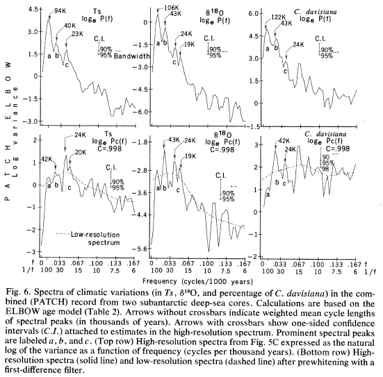
The top graph shows the power spectra for Ts, δ18O, and the percentage of Cycladophora davisiana. The second one shows the spectra after a bit of extra messing around. Either way, there seem to be peaks at frequencies of 19, 23, 42 and roughly 100 thousand years. However the last number is quite fuzzy: if you look, you’ll see the three different power spectra have peaks at 94, 106 and 122 thousand years.
So, some sort of cycles seem to be occurring. This is far from the only piece of evidence, but it’s a famous one.
Now let’s go over the three major forms of Milankovitch cycle, and keep our eye out for cycles that take place every 19, 23, 42 or roughly 100 thousand years!
Eccentricity
The Earth’s orbit is an ellipse, and the eccentricity of this ellipse says how far it is from being circular. But the eccentricity of the Earth’s orbit slowly changes: it varies from being nearly circular, with an eccentricity of 0.005, to being more strongly elliptical, with an eccentricity of 0.058. The mean eccentricity is 0.028. There are several periodic components to these variations. The strongest occurs with a period of 413,000 years, and changes the eccentricity by ±0.012. Two other components have periods of 95,000 and 123,000 years.
The eccentricity affects the percentage difference in incoming solar radiation between the perihelion, the point where the Earth is closest to the Sun, and the aphelion, when it is farthest from the Sun. This works as follows. The percentage difference between the Earth’s distance from the Sun at perihelion and aphelion is twice the eccentricity, and the percentage change in incoming solar radiation is about twice that. The first fact follows from the definition of eccentricity, while the second follows from differentiating the inverse-square relationship between brightness and distance.
Right now the eccentricity is 0.0167, or 1.67%. Thus, the distance from the Earth to Sun varies 3.34% over the course of a year. This in turn gives an annual variation in incoming solar radiation of about 6.68%. Note that this is not the cause of the seasons: those arise due to the Earth’s tilt, and occur at different times in the northern and southern hemispheres.
Obliquity
The angle of the Earth’s axial tilt with respect to the plane of its orbit, called the obliquity, varies between 22.1° and 24.5° in a roughly periodic way, with a period of 41,000 years. When the obliquity is high, the strength of seasonal variations is stronger.
Right now the obliquity is 23.44°, roughly halfway between its extreme values. It is decreasing, and will reach its minimum value around the year 10,000 CE.
Precession
The slow turning in the direction of the Earth’s axis of rotation relative to the fixed stars, called precession, has a period of roughly 23,000 years. As precession occurs, the seasons drift in and out of phase with the perihelion and aphelion of the Earth’s orbit.
Right now the perihelion occurs during the southern hemisphere’s summer, while the aphelion is reached during the southern winter. This tends to make the southern hemisphere seasons more extreme than the northern hemisphere seasons.
The gradual precession of the Earth is not due to the same physical mechanism as the wobbling of the top. That sort of wobbling does occur, but it has a period of only 427 days. The 23,000-year precession is due to tidal interactions between the Earth, Sun and Moon. For details, see:
• John Baez, The wobbling of the Earth and other curiosities.
In the real world, most things get more complicated the more carefully you look at them. For example, precession actually has several periodic components. According to André Berger, a top expert on changes in the Earth’s orbit, the four biggest components have these periods:
• 23,700 years
• 22,400 years
• 18,980 years
• 19,160 years
in order of decreasing strength. But in geology, these tend to show up either as a single peak around the mean value of 21,000 years, or two peaks at frequencies of 23,000 and 19,000 years.
To add to the fun, the three effects I’ve listed—changes in eccentricity, changes in obliquity, and precession—are not independent. According to Berger, cycles in eccentricity arise from ‘beats’ between different precession cycles:
• The 95,000-year eccentricity cycle arises from a beat between the 23,700-year and 19,000-year precession cycles.
• The 123,000-year eccentricity cycle arises from a beat between the 22,4000-year and 18,000-year precession cycles.
We should delve into all this stuff more deeply someday. For now, let me just refer you to this classic review paper:
• André Berger, Pleistocene climatic variability at astronomical frequencies, Quaternary International 2 (1989), 1-14.
Later, as I get up to speed, I’ll talk about more modern work.
Paleontology versus astronomy
So now we can compare the data from ocean sediments to the Milankovitch cycles as computed in astronomy:
• The roughly 19,000-year cycle in ocean sediments may come from 18,980-year and 19,160-year precession cycles.
• The roughly 23,000-year cycle in ocean sediments may come from 23,700-year precession cycle.
• The roughly 42,000-year cycle in ocean sediments may come from the 41,000-year obliquity cycle.
• The roughly 100,000-year cycle in ocean sediments may come from the 95,000-year and 123,000-year eccentricity cycles.
Again, the last one looks the most fuzzy. As we saw, different kinds of sediments seem to indicate cycles of 94, 106 and 122 thousand years. At least two of these periods match eccentricity cycles fairly well. But a detailed analysis would be required to distinguish between real effects and coincidences in this subject!
The effect of eccentricity
I bet some of you are hungry for some actual math. As I mentioned, it takes some work to see how changes in the eccentricity of the Earth’s orbit affect the annual average of sunlight hitting the top of the Earth’s atmosphere. Luckily Greg Egan has done this work for us. While the result is surely not new, his approach makes nice use of the fact that both gravity and solar radiation obey an inverse-square law. That’s pretty cool.
Here is his calculation:
The angular velocity of a planet is

where 


for some constant 
So, the total energy delivered in one period will be

How can we relate the orbital angular momentum 


where
is the semi-major axis of the orbit and

is the semi-minor axis. But we can also relate 

over one orbit. Since the area of an ellipse is 

Equating these two expressions for
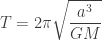
So the period depends only on the semi-major axis; for a fixed value of 
As the eccentricity of the Earth’s orbit changes, the orbital period

Expressing the semi-minor axis in terms of the semi-major axis and the eccentricity, 
So to second order in 

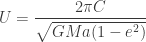
The expressions simplify if we consider average rate of energy delivery over an orbit, which makes all the grungy constants related to gravitational dynamics go away:

or to second order in

We can now work out how much the actual changes in the Earth’s orbit affect the amount of solar radiation it gets! The eccentricity of the Earth’s orbit varies between 0.005 and 0.058. The total energy the Earth gets each year from solar radiation is proportional to

where 
When the eccentricity is at its highest value, 

So, the change is about

In other words, a change of merely 0.167%.
That’s very small And the effect on the Earth’s temperature would naively be even less!
Naively, we can treat the Earth as a greybody: an ideal object whose tendency to absorb or emit radiation is the same at all wavelengths and temperatures. Since the temperature of a greybody is proportional to the fourth root of the power it receives, a 0.167% change in solar energy received per year corresponds to a percentage change in temperature roughly one fourth as big. That’s a 0.042% change in temperature. If we imagine starting with an Earth like ours, with an average temperature of roughly 290 kelvin, that’s a change of just 0.12 kelvin!
The upshot seems to be this: in a naive model without any amplifying effects, changes in the eccentricity of the Earth’s orbit would cause temperature changes of just 0.12 °C!
This is much less than the roughly 5 °C change we see between glacial and interglacial periods. So, if changes in eccentricity are important in glacial cycles, we have some explaining to do. Possible explanations include season-dependent phenomena and climate feedback effects. Probably both are very important!
Next time I’ll start talking about some theories of how Milankovitch cycles might cause the glacial cycles. I thank Frederik De Roo, Martin Gisser and Cameron Smith for suggesting improvements to this issue before its release, over on the Azimuth Forum. Please join us over there.
Little did I suspect, at the time I made this resolution, that it would become a path so entangled that fully twenty years would elapse before I could get out of it. – James Croll, on his decision to study the cause of the glacial cycles


Why does the eccentricity change? If I remember correctly, the eccentricity in the Kepler problem is fixed by 3 parameters: the mass, the angular momentum and the energy of the orbit. So for the eccentricity to change, one of these would have to change. So which is it and why? I suppose I could look it up, but I’m lazy:)
Nice question!
The mass of the Earth and Sun aren’t changing much, so we can treat those as constant and focus on the other parameters determining the shape and size of the Earth’s orbit. In terms of physics, two obvious parameters are energy and angular momentum. In terms of geometry, two obvious parameters are the eccentricity and the semi-major axis, which is this distance:
Apparently the Milankovitch cycles cause changes in the eccentricity without changes in the semi-major axis.
If so, this means that the energy remains constant, while the angular momentum changes. Why? If
then the energy is inversely proportional to the semi-major axis but independent of the eccentricity:
while the angular momentum depends on the semi-major axis and eccentricity as follows:
So, as Milankovitch cycles change the eccentricity of the Earth, the total energy of the Earth-Sun system remains constant, but the angular momentum changes.
Of course there’s another way to answer “why does the eccentricity change?”, and that’s to discuss what interactions actually cause it to change. But I’m not ready for that yet.
I had exactly the same idea, exacerbated by a rule of thumb in mechanics: If something changes, it usually is the energy – conservation of momentum and angular momentum works much “better”. So the real question is “Why do orbital perturbations perturb J but not E?”. In addition, I’d expect the perturbing forces on earth to act mostly radially (other planets pull most strongly if the are in opposition or lower conjunction), and the tangential force contributions before and after that should approximately cancel out.
Ralf wrote:
I don’t know that rule of thumb. Whenever you exert a force on something, its momentum changes, and whenever you exert a torque on it, its angular momentum changes. So your rule of thumb says that in some situations, forces and torques are negligible. But I don’t know which situations those are.
Even though I don’t understand your “rule of thumb”, I agree that this is an interesting question for the changes in the Earth’s orbit!
We’ll need to look at the calculations to see why the semi-major axis, and thus the energy, remains roughly constant while the eccentricity, and thus the angular momentum, changes. Marcel has given us some references over on the Forum:
Thanks for the links ([3] is even available, $a$ changes only by 2.5e-5 there (Fig. 11, p. 15)). The “rule of thumb” comes from my student’s time – there were many homework problems where energy could be either dissipated of transferred into other degrees of freedom, whereas conservation of momentum gives the correct solution. A prototype of such problems is a chain laying on the floor and an end is being lifted with constant speed, and one has to solve for the force needed for lifting. So it is an interesting fact that it is the other way around in celestial mechanics, at least for earth’s orbit; and that one needs real simulations instead of guesswork to arrive there.
Unfortunately, there seems to be some confusion about what the semi-major axis of an ellipse is. Some say (as your picture and the wiki article you link to suggests) that the semi-major axis is one half of the largest axis of the ellipse. Others (like http://en.wikipedia.org/wiki/Orbital_mechanics) define the semi major axis a is the arithmetic mean of the two axes. It is the second definition that corresponds to the energy, not the first one. It does make sense: Suppose that we stopped the earth in its orbit at aphelion and gave it a minor push orthogonal to the direction towards the sun. Then it would drop into the sun. More importantly, it would be on an orbit with the same largest axis as before we stopped it, but with less energy.
Marcel
That push would preserve the aphelion distance, not the semi-major axis (for the simple reason that the perihelion would shrink to zero). The semi-major axis is the arithmetic mean of the aphelion and perihelion distances, maybe the confusion stems from that.
The correct equation ( ) is in the Wikipedia article you cited, in the section on elliptical orbits. Fig. 4 in the article on Kepler’s laws of planetary motion has the correct labels for the variables.
Unfortunately I’m the only one who can include pictures in comments on this blog. So, let me expand a bit on what Ralf said. This figure from the Wikipedia article Kepler’s laws of planetary motion explains the definition of ‘semi-major axis’ and other quantitites:
We see here a planet (the red dot) moving in an elliptical orbit around a much heavier star (the right-hand black dot). The star is at one of the foci of the ellipse; the left-hand black dot is the other focus of the ellipse.
The perihelion is the closest the planet gets to the star. The aphelion
  is the farthest the planet gets from the star. The semimajor axis
  is the arithmetic mean of perihelion and aphelion:
The semi-major axis also has a geometrical meaning: it’s the distance between the ‘center’ of the ellipse (the blue dot) and a point on the ellipse farthest from the center.
The semi-minor axis is the geometric mean of perihelion and aphelion:
The semi-minor axis also has a geometrical meaning: it’s the distance between the center of the ellipse and a point on the ellipse closest to the center.
So, in the picture above, the semi-major axis is half the ‘length’ of the ellipse, while the semi-minor axis is half its ‘height’.
Finally, the most subtle quantity from a geometrical viewpoint is the obscene-sounding semi-latus rectum : this is the length of the segment starting at a focus of the ellipse and going at right angles to the line between the foci until it hits the ellipse. The picture above explains this more clearly than my words!
The advantage of the semi-latus rectum is that the ellipse has a nice formula in polar coordinates involving
  and also the eccentricity
  :
:
If one accepts this, it easily follows that the perihelion is
while the aphelion is
so the semi-major axis is
while the semi-minor axis is
I believe my earlier picture, taken from the Wikipedia article Semi-major axis, correctly shows the semi-major axis:
It is nice that after having learned this stuff and forgotten it many times, it may finally become useful to my actual work!
Oops, here I have been too fast to press the “send” button, sorry about that. But at least I will remember what the semi-major axis is to the end of time…
What about the variation of the orbital plane relative to that of Jupiter (which may contain excess dust)? Has that been discarded as a possible driver?
I don’t think the orbital plane varies significantly over time, but I’ll try to find out as I gradually learn more about this stuff.
I also don’t think interplanetary dust has a significant effect on the Earth’s climate except perhaps as a source of ice nuclei. ‘Ice nuclei’ are particles in the upper atmosphere on which ice forms. They play an important part in the formation of clouds. For a long time the source of most ice nuclei was a mystery. Meteorites were one favored possibility:
• E. K. Bigg and J. Giutronrich, Ice nucleating properties of meteoric material, J. Atmospheric Sciences 24 (1967) 46-49.
However, more recently I think most scientists favor bacteria as the source of most ice nuclei. This is another interesting way in which life on Earth affects the Earth’s climate, perhaps even regulating it to some extent.
it seems there is a slight mistake:
Thanks, nad. I’ll fix that mistake you caught in my comment above.
By the way, it’s sort of fun to prove these formulas for the semi-major axis and semi-minor axis
  :
:
If you stare at this picture:
it’s easy to see that the ‘length’ of the ellipse—the distance between its two farthest points—is the sum
so the semi-major axis is half this:
The semi-minor axis is a bit less obvious, but I figured it out during a bout of insomnia last night. You can draw an ellipse using two pins and piece of string like this:
The total length of the string remains constant as you move your pencil tip around the ellipse. What is the length of the string? When the pencil lies at the far left point of the ellipse, the length of the string is clearly
When the pencil lies at the top point of the ellipse, the length of the string is clearly
where is the hypotenuse of a right triangle formed by a focus of the ellipse, the center of the ellipse, and the top point of the ellipse. So,
On the other hand, by the Pythagorean theorem, this hypotenuse obeys
obeys
where is the horizontal side of the right triangle, and
  is the vertical side.
The vertical side is, by definition, the semi-minor axis! That’s what we want to know.
The horizontal side is the distance between the focus and the center of the ellipse. This is half the distance between the two foci. And if you scratch your head a bit, you’ll see the distance between foci is
so
In summary, we know
and
and
so we can conclude
or with a little algebra
Remembering that is the semi-minor axis, normally called
  , we conclude
The algebra and geometry of ellipses is quite cute; you can see why Apollonius wrote a book on conic sections. But I still think it’s a kind of miracle that the Greeks had developed all this mathematics before Kepler and Newton realized that planets moved in elliptical orbits. If this math hadn’t been ready, it would have been much harder to guess the laws governing gravity. And planets only move around stars in elliptical orbits if the dimension of space is 3.
I am not good at absorbing the math even though I understand it. I always thought that each glacial period started when the earth’s axis was at its greatest obliquity with the northern hemisphere tilting away from the sun during the part of the year the earth was approaching aphelion and leaving it. The northern hemisphere winter would last much longer than the shorter summer at perihelion. This would allow the snow and ice in the north to accumulate to the point that the short summer could not melt it all before the next winter. The albedo of the increasing snow and ice cover would reduce summer melting further. On the flip side, the same thing would not happen in the southern hemisphere because it has more water than the northern hemisphere and water and ocean circulation moderate the air temperature. Here you have eccentricity, obliquity and precession coming together to start an ice age!
Gary wrote:
I’ll say more about different theories later. For now, let me just say that there’s a fair amount of disagreement about exactly how Milankovitch cycles cause the ice ages, and there seems to be a certain amount of random noise involved: no theory I know perfectly explains all the data.
A lot of scientists believe that glacial cycles are correlated to the amount of solar radiation received by the Earth at 65°N in July: that’s the yellow curve below. However, at the very least, it’s not easy to use this curve to predict the Earth’s temperature, as shown in the bottom curve.
How does this affect the amount of incident solar radiation that is re-radiated back into space? I think not at all. I think the absorption characteristics of atmospheric components are well known, as is composition of the incident radiation.
George wrote:
What’s ‘this’?
Here’s a fun puzzle. Use some arithmetic to analyze these statements:
• The 95,000-year eccentricity cycle arises from a beat between the 23,700-year and 19,000-year precession cycles.
• The 123,000-year eccentricity cycle arises from a beat between the 22,4000-year and 18,000-year precession cycles.
What’s the big difference between these two claims?
1/19 − 1/23.7 = 1/96
1/18 − 1/22.4 = 1/92 ≠ 1/123
Am I warm?
In Statistics 101 we learn that correlations do not prove causes, and the complete inability to explain the cause of the correlation for the alleged connection between orbital variations and climate is unexplainable. Well actually, it is explainable as being coincidence, since the odds of so very many variations in orbital variations coinciding with climate change is very high. Any “theory” which tries to link these correlations to a cause are bordering on pseudo-science, since these same exact orbital variations also existed for millions of years BEFORE the current Ice Age started up about 4 million years ago.
For a serious and scientifically sound attempt at explaining the current Ice Age, especially the timing, see
Sea ice switch mechanism and glacial-interglacial CO 2 variations,
by Hezi Gildor and Eli Tziperman
Interesting, they also released another (earlier) paper in which they discussed this sea ice switch mechanism in conjunction with orbital forcing
Sea ice as the glacial cycles’ climate switch: Role of seasonal and orbital forcing, by Hezi Gildor and Eli Tziperman
Now while they call it a “forcing” it is more accurately described as a trigger and not a cause, much in the same way that Maunder Minimums can trigger colder weather but do not cause colder weather.
Here is a brief summary of some time series analysis I performed in order to better understand the relationship between the Earth’s Ice Ages and the Milankovich cycles. […]