I wish you all happy holidays! My wife Lisa and I are going to Bangkok on Christmas Eve, and thence to Luang Prabang, a town in Laos where the Nam Khan river joins the Mekong. We’ll return to Singapore on the 30th. See you then! And in the meantime, here’s a little present—something to mull over.

Statistical mechanics versus quantum mechanics
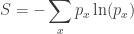
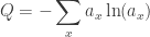
There’s a famous analogy between statistical mechanics and quantum mechanics. In statistical mechanics, a system can be in any state, but its probability of being in a state with energy 

where 

where 
| Statistical Mechanics | Quantum Mechanics |
| probabilities | amplitudes |
| energy | action |
| temperature | Planck’s constant times i |
In other words, making the replacements


formally turns the probabilities for states in statistical mechanics into the amplitudes for paths, or ‘histories’, in quantum mechanics.
But the probabilities 

Following the analogy without thinking too hard, we’d guess it arises from minimizing something subject to a constraint on the expected action.
But now we’re dealing with complex numbers, so ‘minimizing’ doesn’t sound right. It’s better talk about finding a ‘stationary point’: a place where the derivative of something is zero.
More importantly, what is this something? We’ll have to see—indeed, we’ll have to see if this whole idea makes sense! But for now, let’s just call it ‘quantropy’. This is a goofy word whose only virtue is that it quickly gets the idea across: just as the main ideas in statistical mechanics follow from the idea of maximizing entropy, we’d like the main ideas in quantum mechanics to follow from maximizing… err, well, finding a stationary point… of ‘quantropy’.
I don’t know how well this idea works, but there’s no way to know except by trying, so I’ll try it here. I got this idea thanks to a nudge from Uwe Stroinski and WebHubTel, who started talking about the principle of least action and the principle of maximum entropy at a moment when I was thinking hard about probabilities versus amplitudes.
Of course, if this idea makes sense, someone probably had it already. If you know where, please tell me.
Here’s the story…
Statics
Static systems at temperature zero obey the principle of minimum energy. Energy is typically the sum of kinetic and potential energy:

where the potential energy 


This is actually somewhat surprising: usually minimizing the sum of two things involves an interesting tradeoff. But sometimes it doesn’t!
In quantum physics, a tradeoff is required, thanks to the uncertainty principle. We can’t know the position and velocity of a particle simultaneously, so we can’t simultaneously minimize potential and kinetic energy. This makes minimizing their sum much more interesting, as you’ll know if you’ve ever worked out the lowest-energy state of a harmonic oscillator or hydrogen atom.
But in classical physics, minimizing energy often forces us into ‘statics’: the boring part of physics, the part that studies things that don’t move. And people usually say statics at temperature zero is governed by the principle of minimum potential energy.
Next let’s turn up the heat. What about static systems at nonzero temperature? This is what people study in the subject called ‘thermostatics’, or more often, ‘equilibrium thermodynamics’.
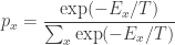
In classical or quantum thermostatics at any fixed temperature, a closed system will obey the principle of minimum free energy. Now it will minimize

where 
But where does the principle of minimum free energy come from?
One nice way to understand it uses probability theory. Suppose for simplicity that our system has a finite set of states, say 


The expected value of the energy is

Now suppose our system maximizes entropy subject to a constraint on the expected value of energy. Thanks to the Lagrange multiplier trick, this is the same as maximizing

where 

This is just a calculation; you must do it for yourself someday, and I will not rob you of that joy.
But what does this mean? We could call 


(For negative temperatures, maximizing
So, every minimum or maximum principle described so far can be seen as a special case or limiting case of the principle of maximum entropy, as long as we admit that sometimes we need to maximize entropy subject to constraints.
Why ‘limiting case’? Because the principle of least energy only shows up as the low-temperature limit, or 
Dynamics
Now suppose things are changing as time passes, so we’re doing ‘dynamics’ instead of mere ‘statics’. In classical mechanics we can imagine a system tracing out a path 


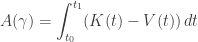
where 


The principle of least action says that if we fix the endpoints of this path, that is the points 

Why is there a minus sign in the definition of action? How did people come up with principle of least action? How is it related to the principle of least energy in statics? These are all fascinating questions. But I have a half-written book that tackles these questions, so I won’t delve into them here:
• John Baez and Derek Wise, Lectures on Classical Mechanics.
Instead, let’s go straight to dynamics in quantum mechanics. Here Feynman proposed that instead of our following a single definite path, it can follow any path, with an amplitude 
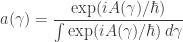
where 
Unfortunately the integral over all paths—called a ‘path integral’—is hard to make rigorous except in certain special cases. And it’s a bit of a distraction for what I’m talking about now. So let’s talk more abstractly about ‘histories’ instead of paths with fixed endpoints, and consider a system whose possible ‘histories’ form a finite set, say 
Suppose the action of the history 


This looks very much like the Boltzmann distribution:
Indeed, the only serious difference is that we’re taking the exponential of an imaginary quantity instead of a real one.
So far everything has been a review of very standard stuff. Now comes something weird and new—at least, new to me.
Quantropy
I’ve described statics and dynamics, and a famous analogy between them, but there are some missing items in the analogy, which would be good to fill in:
| Statics | Dynamics |
| statistical mechanics | quantum mechanics |
| probabilities | amplitudes |
| Boltzmann distribution | Feynman sum over histories |
| energy | action |
| temperature | Planck’s constant times i |
| entropy | ??? |
| free energy | ??? |
Since the Boltzmann distribution
comes from the principle of maximum entropy, you might hope Feynman’s sum over histories formulation of quantum mechanics:
comes from a maximum principle too!
Unfortunately Feynman’s sum over histories involves complex numbers, and it doesn’t make sense to maximize a complex function. However, when we say nature likes to minimize or maximize something, it often behaves like a bad freshman who applies the first derivative test and quits there: it just finds a stationary point, where the first derivative is zero. For example, in statics we have ‘stable’ equilibria, which are local minima of the energy, but also ‘unstable’ equilibria, which are still stationary points of the energy, but not local minima. This is good for us, because stationary points still make sense for complex functions.
So let’s try to derive Feynman’s prescription from some sort of ‘principle of stationary quantropy’.
Suppose we have a finite set of histories, 

since that’s what Feynman’s normalization actually achieves. We can try to define the quantropy of 
You might fear this is ill-defined when 

and everything works fine. The worst problem is that the logarithm has different branches: we can add any multiple of 

Next, suppose each history 


The term ‘expected action’ is a bit odd, since the numbers
So, let’s look for a stationary point of 
But there’s another constraint, too, namely
So let’s write

and look for stationary points of
To do this, the Lagrange multiplier recipe says we should find stationary points of

where 


This says that when
So, we’ll follow the usual Lagrange multiplier recipe and look for amplitudes for which

holds, along with the constraint equations. We begin by computing the derivatives we need:
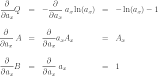
Thus, we need

or
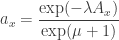
The constraint

then forces us to choose:

so we have

Hurrah! This is precisely Feynman’s sum over histories formulation of quantum mechanics if
We could go further with the calculation, but this is the punchline, so I’ll stop here. I’ll just note that the final answer:

does two equivalent things in one blow:
• It gives a stationary point of quantropy subject to the constraints that the amplitudes sum to 1 and the expected action takes some fixed value.
• It gives a stationary point of the free action:

subject to the constraint that the amplitudes sum to 1.
In case the second point is puzzling, note that the ‘free action’ is the quantum analogue of ‘free energy’, 


Note also that when
Summary. We recover Feynman’s sum over histories formulation of quantum mechanics from assuming that all histories have complex amplitudes, that these amplitudes sum to one, and that the amplitudes give a stationary point of quantropy subject to a constraint on the expected action. Alternatively, we can assume the amplitudes sum to one and that they give a stationary point of free action.
That’s sort of nice! So, here’s our analogy chart, all filled in:
| Statics | Dynamics |
| statistical mechanics | quantum mechanics |
| probabilities | amplitudes |
| Boltzmann distribution | Feynman sum over histories |
| energy | action |
| temperature | Planck’s constant times i |
| entropy | quantropy |
| free energy | free action |


[…] Baez introduces a notion of “quantropy” which is supposed to be a quantum-dynamical analogue to entropy in statistical […]
The weirdest part of this story for me is not the notion of “quantropy”. Rather, it’s that in statistical mechanics, one sometimes treats the temperature T is a dynamical variable itself. I don’t know of any context in quantum mechanics / field theory where is a dynamical variable. A variable, sure, but not one that varies with other dynamical variables.
Of course, I’d probably need an extra time dimension.
I agree, one of the peculiar things about this analogy is that temperature is something we can control, but not Planck’s constant… except for mathematical physicists, who casually use their superhuman powers to “set Planck’s constant to one” or “let Planck’s constant go to zero”.
There are some rather strange papers that treat Planck’s constant as a variable and even quantize it, but I can’t find them now—all I can find are some crackpot websites that discuss the quantization of Planck’s constant. The difference between ‘strange papers’ and ‘crackpot websites’ is that the former do mathematically valid things without making grandiose claims about their physical significance, while the latter make grandiose claims without any real calculations to back them up. Anyway, all this is too weird for me, at least today.
Somewhat less weird, but still mysterious to me, is the analogy between canonically conjugate variables in classical mechanics, and thermodynamically conjugate variables in thermodynamics. Both are defined using Legendre transforms, but I want to figure out more deeply what’s going on here. I mention this only because it might shed light on the idea of temperature as a dynamical variable.
Consider the following sequence of steps: (0) conjugate pair (q,p); (1) canonical 1-form p dq; (2) “kinematic law” v = dq/dt; (3) “dynamic law” f = dp/dt; (4) Lagrangian form as Lie derivative dL = Lie_{d/dt} (p dq) = f dq + p dv; (5) select out a subset (F, Q) of (f, q) coordinates; (6) lump the average of the remaining (f,q)’s and all the (p,v)’s into T dS to get the thermodynamic form T dS + F dQ; (8) for the p-V systems Q: {V}, F: {-p} this reduces to T dS – p dV.
For the Legendre transform (9) take the canonical 2-form dq dp (wedge products denoted by juxtaposition); (10) contract d/dt with this to obtain v dp – dq f = dH … the Hamiltonian form; (11) the formula for the Lie derivative is one and the same as the Legendre transform; (12) to apply this directly to the reduction done in (5) would require a time integral U for the temperature T, if treating S as one of the Q’s. Then the analogue of the canonical 1-form would be U dS + P dQ, with “dynamic law” dU/dt = T, dP/dt = F.
Slightly off topic but those notes on classical mechanics are fantastic. Thanks! I wish I had seen explanations that clear the first, or 2nd or 3rd, times I was taught Hamiltonian/Lagrangian Mechanics.
Thanks a million!
Me too!
It’s taken me decades to understand this stuff. I guess I really should finish writing this book.
Yeah. I’ve almost forgotten about these yummy lectures – They are in my huge pile of undone homework, much of it inspired by grandmaster John… I need to get 100 years old, it looks.
I am surprised you did not mention Wick rotations.
Wick rotations.
In quantum information theory, there’s already a notion of “quantum” entropy, aka the von Neumann entropy, defined as the “entropy function” applied to the set of eigenvalues of a density matrix. How does that compare to what you describe here ?
For more info, Watrous’ lecture notes are great: http://www.cs.uwaterloo.ca/~watrous/quant-info/lecture-notes/07.pdf
Yes, there’s a perfectly fine concept of entropy for quantum systems, the von Neumann entropy, which is utterly different from ‘quantropy’. Quantropy is not entropy for quantum systems!
In my analogy charts I’m comparing
• statics at nonzero temperature and zero Planck’s constant (‘classical equilibrium thermodynamics’)
to
• dynamics at zero temperature and nonzero Planck’s constant (‘quantum mechanics’)
Entropy has a starring role in the first subject, and quantropy seems to be its analogue in the second.
Von Neumann entropy shows up as soon as we study
• statics at nonzero temperature and nonzero Planck’s constant (‘quantum equilibrium thermodynamics’)
Just as a classical system in equilibrium at nonzero temperature maximizes entropy subject to a constraint on the expected energy, so too a quantum system in equilibrium at nonzero temperature maximizes von Neumann entropy subject to a constraint on the expected energy.
So, one interesting question is how the analogy I described might fit in a bigger picture that also includes
• dynamics at nonzero temperature and nonzero Planck’s constant (‘quantum nonequilibrium thermodynamics’)
But, I don’t know the answer!
One small clue is that my formula for the Boltzmann distribution
while phrased in terms of classical mechanics, also works in quantum mechanics if is the set of energy eigenstates and
  are the energy eigenvalues. The probabilities
  are then the diagonal entries of a density matrix, and its von Neumann entropy is just what I wrote down:
So, the first column in my analogy chart, which concerns classical equilibrium thermodynamics, already contains some of the necessary math to handle quantum equilibrium thermodynamics.
If you think this is a bit confusing, well, so do I. I don’t think we’ve quite gotten to the bottom of this business yet.
Ah I see. Clearly I didn’t understand the original post, and your comment helps clarify the differences very nicely.
Great post, I am sure it will spark some discussion on the merits and history of quantropy and related thoughts over the holidays, so the timing is great. The anology between temperature and planck’s constant is a fun one to play with, bringing up thoughts of equilibrium conditions. A lot of fun thought to be had on this one.
Just noticed a typo on page 3 of the Lectures on Classical Mechanics: near the bottom it says when it means
  .
.
Thanks, I fixed that! If anyone else spots typos or other mistakes, please let me know and I’ll fix them.
By the way, the tone of voice of this book is one thing I want to work on in future draft, since while it’s based on notes from my lectures, most of the actual sentences were written by Blair Smith, who LaTeXed it. It doesn’t sound like me—so sometime I’ll need to change it so it does.
The $F_{\mu \nu}$ in (3.4) should be a $F_{ij}$. (Nice book BTW!)
Damn, now I gotta TeX the whole thing again! I just did it 10 minutes ago.
But thanks!
Very nice. I’ve pointed you to my http://arxiv.org/abs/quant-ph/0411156v2, doi:10.1016/j.physleta.2005.02.019 before (https://johncarlosbaez.wordpress.com/2010/11/02/information-geometry-part-5/#comment-2316), where section 4 establishes that, for the free KG field, we can think of Planck’s constant as a measure of the amplitude of Lorentz invariant fluctuations — in contrast to the temperature, which we can think of as a measure of the amplitude of Aristotle group invariant fluctuations (of the Aristotle Group, see your comments at the link).
So, quantropy, which is a nice coining, is a measure of Lorentz invariant fluctuations, where entropy is a measure of Aristotle group invariant fluctuations (which is a nicely abstract enough definition to encourage me to hope that the free field case will extend to the interacting case). However, in my thinking it has been hard to see the relationship between quantropy and entropy as straightforward because of the appearance of the factor in a presentation of the thermal state of a free quantum field; whereas I could see your extremization approach yielding a more natural relationship through the relationship between two group structures.
Although Feynman’s path integral approach has ruled QFT for so long, it can be understood to be no more than a way to construct a generating function for VEVs, which are more-or-less closely related to observables. Nothing says that a generating function has to be complex, even though there are certainly advantages to taking that step. My feeling is that if we use some other type of transform that the one introduced by Feynman (the Feynman VEV transform?), your relationship would look different. In particular, we could hope that we could write instead of
  .
.
This analogy works perfectly, provided one is willing to swallow complex probabilities for paths — which requires a lot of chewing. I think the most interesting aspects are how the wavefunction arises as the square root of that probability, due to time reversibility of the action, and the fact that you can explicitly write down the probability distribution over paths, and not just the partition function, and use it to calculate expectation values.
I wrote up a description in 2006, and nobody, including me, has talked about it much:
http://arxiv.org/abs/physics/0605068
Thanks, Garrett! I hadn’t known about that paper—it looks more like what I’m talking about than anything I’ve ever seen! If I ever publish this stuff I’ll definitely cite it. I see nice phrases like ‘expected path action’ and:
My own attitude is that it’s more useful to treat amplitudes as analogous to probabilities than one would at first think (since probabilities are normally computed as the squares of absolute values of amplitudes), and that this is yet another bit of evidence for that. After my recent talk about this analogy people asked:
• What are some ways you can use your analogy to take ideas from quantum mechanics and turn them into really new ideas in stochastic mechanics?
and
• What are some ways you can use it in reverse, and take ideas from stochastic mechanics and turn them into really new ideas in quantum mechanics?
and I think this ‘quantropy’ business is an example of the second thing.
Thanks, John, I’d be delighted if you get something out of these ideas. You’d be the first to cite that paper of mine. I consider it to be based on kind of a crazy idea, but maybe the kind of crazy that’s true.
The biggest weirdness is allowing probabilities (in this case, of paths) to be complex. Once you do that, and allow your system paths to be in an action bath, described by Planck’s constant in the same way that a canonical ensemble is in a temperature bath, then everything follows from extremizing the entropy subject to constraints.
I had the same exciting idea: lots of interesting stat mech techniques could be brought to bare on questions in quantum mechanics. And I still think that’s true. I would have worked on this more, but got distracted with particle physics unification stuff. The most exciting thing, I think, is having a direct expression for the probability of a path (eq 2 in the paper), and not just having to deal with the usual path integral partition function.
There’s a lot of neat stuff here. I hadn’t even thought of classical, physics as being analogous to the zero temperature limit. Cool.
But, although I believe our thinking on this is based on the same basic analogy, we seem to be departing on our interpretation of what the quantum amplitude (wavefunction) is and where it is coming from. For me, I’m extremizing the usual entropy as a functional of the probability of paths to get the (complex, bizarrely) probability distribution. This is not the usual quantum amplitude, but the actual probability distribution. When one tries to use this to calculate an expectation value, or the probability of a physical outcome, one gets a real number. And when one looks at a system with time independence, the probability of an event breaks up into the amplitude of incoming paths and outgoing paths, multiplied. So that is the usual quantum amplitude (wavefunction) squared to get probability.
So… I guess we differ in that I think the only really weird thing one needs to do is accept the idea of complex probabilities of paths, and then use entropy extremization in the usual way to determine the probability distribution (finding the probability distribution compatible with our ignorance), rather than defining quantropy to determine amplitudes. It’s currently too late here in Maui for me to figure out to what degree quantropy will give equivalent results… but I suspect only for time independent Lagrangians, if those. Also, quantropy and amplitudes require some new rules for calculating things, whereas we know how to use a probability distribution to calculate. In any case though, whichever approach is correct, I agree this is a fascinating analogy that warrants more attention.
Hi Garret, , then the upper limit of the second integral should also be
  . Similarly in the product of integrals in the 6th equation, it seems both the lower limit of the first and the upper limit of the second should be
  . But this seems to conflict with your interpretation of the second integral being associated with paths for
  . Is this why you require the system to be time-symmetric?
In your paper, in the 5th equation on p.3, if the lower limit of the first integral is
Jim, ironically enough, there’s no reply button beneath your comment, so this reply appears time reversed. Yes, for this to work, must be time independent. Then the action of paths coming in to some point,
  , is equal to the negative of the action of paths leaving it.
This reminds me of a reformulation of the path integral formulation given by Sinha and Sorkin
(www.phy.syr.edu/~sorkin/some.papers/63.eprb.ps, eq.(2.4) and preceding text). They rewrite the absolute square of the sum over paths, which gives the total probability for some position measurement, as a sum of products of amplitudes with complex-conjugated amplitudes. They then interpret the complex conjugates as being associated with time-reversed, incoming paths, as opposed to your time-forward, outgoing paths; but both interpretations should be equally valid for a time-independent Lagrangian. Their amplitudes also seem more properly interpreted as probabilities, albeit complex, with their products representing conjunction.
Jim, yes, it does appear to be compatible with the forward and backwards histories approach in Sinha and Sorkin’s paper. Thanks for the link.
I wonder whether the concept of complex probability can be made rigorous.
Jim wrote:
Everything I’m doing in my blog article is perfectly rigorous, and it involves a bunch of complex numbers that sum to one. But I prefer not to call them ‘probabilities’, because probability theory is an established subject, and we’d be stretching the word in a drastic way.
But the terminology matters less than the actual math. A lot of new problems show up. For example, quantropy is not well-defined until we choose a branch for the logarithm function in this expression:
After we do this, everything in this blog article works fine, but it’s still unnerving, and I’m not quite sure what the best way to proceed is. One possibility is to decree from the start that $s_x = \ln a_x$ rather than is the fundamentally important quantity, and then define quantropy by
This amounts to picking a logarithm for each number once and for all from the very start. To handle the possibility that
  , we have to say that
  is allowed.
I guess I was really wondering whether we could consider this a complex generalization of conventional probability theory. Another paper suggests this is possible:
Click to access complex-prob.pdf
They define complex probability in the context of a classical Markov chain. Their complex probabilities also sum to 1.
Hmm – thanks for that reference, Jim! I’ve seen work on ‘quantum random walks’ but not on ‘complex random walks’ where the complex probabilities sum to 1!
Jim, some things to consider: John and my descriptions differ slightly. I use the usual entropy, in terms of a (weird) complex probability over paths, in the presences of an h background. John instead defines a new thing, quantropy, in terms of amplitudes. I don’t know how rigorous one can make complex probabilities. Good question. I find it somewhat reassuring that when calculating the probability of any physical event from these complex probabilities, the result is real.
There’s also Scott Aaronson’s great article on various reasons why complex numbers show up in QM.
http://www.scottaaronson.com/democritus/lec9.html
Btw, I think it’s a bit suboptimal for you to post comments as “repieriendi” instead of Mike Stay, especially comments that would help build the “Mike Stay” brand (knowledgeable about quantum theory, etc.).
Best, jb
Thanks—I just discovered that I can change the “display name” on my WordPress account so it shows my name instead of my username.
This question is pure crackpottery, but it’s not like I was fooling anyone anyway so here goes.
If time’s arrow is also the arrow of thermodynamics, and if the second law is routinely “violated” at small scales subject to the fluctuation theorem, doesn’t that practically beg that causality can also be violated at those scales? It makes me wonder whether these complex probabilities actually represent the combined real probabilities of casual and anti-casual paths. In this case the difference between stochastic and quantum mechanics would be whether to consider such paths.
One day I should learn math. Thanks for the blog.
Do you see the account here fitting in with the matrix mechanics over a rig we used to talk about?
Perhaps here is the best place to see that conversation.
All my recent work on probabilities versus amplitudes is about comparing matrix mechanics over the ring of complex numbers to matrix mechanics over the rig of nonnegative real numbers. The first is roughly quantum mechanics, the second roughly stochastic mechanics—but this only becomes true when we let our matrices act as linear transformations of Hilbert spaces in the first case and spaces in the second. In other words, what matters is not just the rig but the extra structure with which we equip the modules over this rig.
I’ve been spending a lot of time taking ideas from quantum mechanics and transferring them to stochastic mechanics. But now, with this ‘quantropy’ business, I’m going the other way.
Thinking of the the principal of least action in terms of matrix mechanics over the tropical rig, which has + as its ‘multiplication’ and min as its ‘addition’—that’s another part of the picture. Maybe that’s what you’re actually asking about. But as you know, the tropical rig only covers the limit of equilibrium thermodynamics. Here I’m trying to think about the
  case and also the imagary-
 case all in terms of ‘minimum principles’, or at least ‘stationary principles’.
I suppose more focused questions might elicit more coherent answers!
Something I’m a little unclear on is how you view the relationship between statistical mechanics and stochastic mechanics. Are they just synonyms?
And then there’s the need for two parameters. Remember once you encouraged me to think of temperatures living on the Riemann sphere.
David wrote:
No, not for me.
I use ‘statistical mechanics’ as most physicists do: it’s the use of probability theory to study classical or quantum systems for which one has incomplete knowledge of the state.
So, for example, if one has a classical system whose phase space is a symplectic manifold , we use a point in
  to describe the system’s state when we have complete knowledge of it—but when we don’t, we resort to statistical mechanics and use a probability distribution on
  , typically the probability distribution that maximizes entropy subject to the constraints provided by whatever we know. A typical example would be a box of gas, where instead of knowing the positions and velocities of all the atoms, we only know a few quantities that are easy to measure. The dynamics is fundamentally deterministic: if the system is in some state
  at some initial time, it’ll be in some state
  at time
  , where
  is a function from
  to
to  . But if we only know a probability distribution to start with, that’s the best we can hope to know later.
There is also quantum version of the last paragraph: statistical mechanics comes in classical and quantum versions, and the latter is what we need when we get really serious about understanding matter as made of zillions of atoms, or radiation as made of zillions of photons.
Stochastic mechanics, on the other hand, is a term I use to describe systems where time evolution is fundamentally nondeterministic. More precisely, in stochastic mechanics time evolution is described by a Markov chain (if we think of time as coming in discrete steps) or Markov process (if we think of time as a continuum). So, the space of states can be any measure space , and if we start the system in a state
  at some initial time, the state will be described by a probability measure on
  .
.
I introduced the term stochastic mechanics in my network theory course because I wanted to spend a lot of time discussing a certain analogy between quantum mechanics and stochastic mechanics—so I wanted similar-sounding names for both subjects. Other people may talk about ‘stochastic mechanics’, but I don’t take any responsibility for knowing what they mean by that phrase.
Since they both involve probability theory, statistical mechanics and stochastic mechanics are related in certain ways (which I haven’t tried very hard to formalize). But I think of them as different subjects.
But why then up above do you say that quantropy is an example of an answer to
when the whole post was on an analogy between statistical mechanics and quantum mechanics?
Jaynesian/de Finettians would not see much of a difference, since for them probabilities only emerge due to our ignorance. In the stochastic mechanics case, when you specify a state, that’s really a macrostate covering a huge number of microstates. In that different microstates will evolve into non-equivalent microstates, there’s your nondeterministic evolution. But presumably in statistical mechanics, microstates of the same macrostate can diverge into different macrostates too.
David wrote:
You’re right, I could have phrased this discussion in terms of stochastic mechanics. I guess I should try it! But in this blog post I preferred to talk about statistical mechanics.
What’s the difference?
In this blog post you’ll see there’s no mention of dynamics, i.e., time evolution, in my discussion of the left side of the chart: the statistical mechanics side. I am doing statics on the left side of the chart, but dynamics on the right side of the chart: the quantum side. We’re seeing an analogy between statics at nonzero temperature and zero Planck’s constant, and dynamics at nonzero Planck’s constant and zero temperature.
On the other hand, my analogy between stochastic mechanics and quantum mechanics always involves comparing stochastic dynamics, namely Markov processes, to quantum dynamics, namely one-parameter unitary groups.
So I think of these as different stories. But your words are making me ashamed of not trying to unify them into a single bigger story. And indeed this must be possible.
One clue, which you mentioned already, is that we need to allow both temperature and Planck’s constant be nonzero to see the full story.
There are lots of other clues.
I guess statistical mechanics is the kind of dynamics where because of a good choice of equivalence relation, change is largely confined to movement within one class, hence it appears to be a statics. Your stochastic dynamics doesn’t typically respect the equivalence classes of a certain number of rabbits and wolves being alive.
David wrote:
I wouldn’t say that. I don’t want to say what I would say, because it’d be long. But:
1) For a certain class of stochastic dynamical systems, entropy increases as time runs, and the state approaches a ‘Gibbs state’: a state that has maximum entropy subject to the constraints provided by the expected values of the conserved quantities. Gibbs states are a big subject in statistical mechanics, and the Boltzmann distribution I’m discussing here is a Gibbs state where the only conserved quantity involved is energy.
2) On the other hand, statistical mechanics often studies Gibbs states, not for stochastic dynamical systems, but for deterministic ones, like classical mechanics.
In your first box you mention the analogy between energy (statistical mechanics) and action (quantum theory). At first glance (and as a wild guess), that looks like some sort of Legendre transform. Can one can get from one to the other by a certain Legendre transform? That would be nice.
Doing a quick search I see that you mention Legendre transforms in response to Theo’s comment. So maybe I am not too far off. On the other hand you might have considered and discarded that already.
I’ll think about this, thanks. Right now I’m in the airport in Bangkok. Bad keyboard.
Merry Christmas!
OK, so I read this, and thought, “oh John is jumping to conclusions, what he should have done is this: normalize with and take
 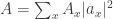 just like usual in QM, and then he should derive Q…” and so I sat down to do this myself, and quickly realized that, to my chagrin, that Feynman’s path amplitude doesn’t obey that sum-of-squares normalization. Which I found very irritating, as I always took it for granted, and now suddenly it feels like a very strange-looking beast.
Any wise words to explicate this? Clearly, what I tried to do fails because I’m mixing metaphors from first & second quantization. But why? Seems like these metaphors should have been more compatible. I’m not even sure why I’m bothering to ask this question…
Merry Christmas, Linas! I successfully made it to Luang Prabang.
I don’t have any wise words to explicate why the Feynman path integral is normalized so that the amplitudes of histories sum to 1:
instead of having
I just know that this is how it works, and this is how it has always worked. But I agree that it seems weird, and I want to understand it better. It’s yet another interesting example of how sometimes it makes sense to treat amplitudes as analogous to probabilities, without the absolute value squared getting involved. This is a theme I’ve been pursuing lately, but mainly to take ideas from quantum mechanics and apply them to probability theory. This time, with ‘quantropy’, I’m going the other way—and at some point I realized that the path integral approach is perfectly set up for this.
I wouldn’t say that. I might say you’re mixing metaphors from the Hamiltonian (Hilbert space) approach to quantization and the Lagrangian (path integral) approach. Both can be applied to first quantization, e.g. the quantization of particle on a line! But somehow states like to have amplitudes whose absolute values squared sum to one, while histories like to have amplitudes that sum to one.
Now I dare ask about that little distraction: Doing the path integral in general. I found this quite a fascinating problem in a former life, but never made it to any closer inspection. It smells like quite a fundamental thing.
Wandering off-topic a bit further, I’d like to mention that probabilities & amplitudes generalize to geometric values (points in symmetric spaces) in general. Some years ago, I had fun drafting the Wikipedia article http://en.wikipedia.org/wiki/Quantum_finite_automata when a certain set of connections gelled (bear with me here). A well-known theorem from undergrad comp-sci courses is that deterministic finite automata (DFA) and probabilistic finite automata (PFA) are completely isomorphic. In a certain sense, the PFA is more-or-less a set of Markov chains. What’s a Markov chain? Well, a certain class of matricies that act on probabilities; err, a vector of numbers totaling to one, err, a simplex, viz an N-dimensional space such that
Some decades ago, someone clever noticed that you could just replace the simplex by and the Markov matrix by elements taken from
  while leaving the rest of the theory untouched, and voila, one has a “quantum finite automaton” (QFA). This generalizes obviously: replace probabilities by some symmetric space in general, and replace the matrices by automorphisms of that space (the “geometric FA” or GFA). Armed with this generalization, one may now ask the general question: how do the usual laws & equations of stat-mech and QM and QFT generalize to this setting?
A few more quick remarks: what are the elements remaining in common across the PFA/QFA/GFA? Well, one picks an initial state vector from the space, and one picks out a hand-full of specific automorphisms from the automorphism group. Label each automorphism by a symbol (i.e. index) Then one iterates on these (a la the Barnsley fractal stuff!) There’s also a “final state vector”. If the initial state vector, after being iterated on by a finite number of these xforms, matches the final vector, then the automaton “stops”, and the string of symbols belongs to the “recognized language” of the automaton. (The Barnsley IFS stuff has a ‘picture’ as the final state, and the recognized language is completely free in the N symbols: all possible sequences of the iterated matrixes are allowed/possible in IFS).
You also wrote about graph theory/network theory (which I haven’t yet read) but I should mention that one may visualize some of the above via graphs/networks, with edges being automorphisms, etc. And then there are connections to model theory… Anyway, I find this stuff all very fascinating, wish I had more time to fiddle with it. I’m mentioning this cause it seems to overlap with some of your recent posts.
OH, and BTW, as far as I can tell, this is an almost completely unexplored territory; there are very few results. I think that crossing over tricks from physics and geometry to such settings can ‘solve’ various unsolved problems, e.g. by converting iterated sequences into products of operators. and back, and looking for the invariants/conserved quantities associated with the self-similarity/translation-invariance. Neat stuff, I think…
Oh! It’s a guess, but probably the difference arises because what matters in a state is the measurements you can subject it to, but when taking sum over histories, we’re applying linear operators and not measuring anything until all the interactions are turned off.
If you want to learn about path integrals, Florifulgurator, I suggest Barry Simon’s book Functional Integration and Quantum Physics. I wouldn’t suggest this for most people, but I get the impression you like analysis and like stochastic processes! This features both. And it’s well-written, too, though it assumes the reader has taken some graduate-level courses on real analysis and functional analysis. It focuses on what we can do rigorously with path integrals, which is just a microscopic part of the subject, but still very interesting. The rest is ‘mathemagical’ technology that I hope will be made rigorous sometime in this century.
There is a vivid geometric realization of complex time that enters in through the back door by way of considering the question of how relativity and non-relativistic theory are related to one another.
The question is not merely academic. The FRW metric, for instance, has the form where
where  approaches 0 as we approach the Big Bang singularity. This is nothing less than a cosmological realization of the Galilean limit. Thus, all three issues are intertwined: complex time, the Big Bang and the Galilean limit.
So, consider the relativistic mass shell invariant . Replace the total energy
  and invariant mass $m$ by the kinetic energy
  and relativistic mass
  . Then the invariant becomes
  and the mass shell constraint reduces to the form
  . This is a member of the family
[…]
invariants parametrized by ; where
  for relativity, and
  for non-relativistic theory and
  , Galilean when
  and locally Euclidean when
  ), while
  shadows the flow of absolute time on the 4-D manifold itself. For instance, a 5-D worldline is projected onto each 4-D layer as an ordinary worldline. But there is one additional feature: the intersection of the projected worldline with the actual worldline singles out a single instant in time: a "now".
Sorry, the reply got cut off in mid-section and restitched, with most of the body lost. I’ll try this again later.
The above comment can also be read here, nicely formatted:
http://www.docstoc.com/docs/109661975/ThermoTime
Everyone please remember: on all WordPress blogs, LaTeX is done like this:
$latex E = mc^2$
with the word ‘latex’ directly following the first dollar sign, no space. Double dollar signs and other fancy stuff don’t work here, either!
Thanks for your help. It’s probably best to go to the web link. The sentence starting out “This is a member” in the reply above is chopped off and ends with a fragment that comes from the end of the reply, with the middle 6-7 paragraphs lost. It may be a coincidence that the Frankenedited sentence almost makes sense — or it may be the blog-compiler is starting to understand language.
I’ve inserted a
[…]
in your post, Mark, to make it obvious that it’s not supposed to make sense around there. If you email the TeX I’ll be happy to fix the darn thing, since I like having the conversation here rather than dispersed across the web, and I like having comments that make sense!
(Perhaps emboldened by your fractured comment, but more likely just by the silly word ‘quantropy’ and the grand themes we’re discussing here, I’ve gotten a few comments that were so visionary and ahead of their time I’ve had to reject them.)
Your actual comment seems quite neat, but it’s raising a tangential puzzle in my mind, which is completely preventing me from understanding what you’re saying.
You start by pointing out that the speed of light essentially goes to infinity as we march back to the Big Bang, making special relativity reduce to Galilean physics. But ‘the speed of light’ here is a rather tricky coordinate-dependent concept: you’re defining it to be in coordinates where the metric looks like this:
Then, since as
as  in the usual Big Bang solutions, we get
  .
.
On the other hand, there’s a fascinating line of work going back to Belinskii, Khalatnikov and Lifshitz which seems to present an opposite picture: one in which each point of space becomes essentially ‘isolated’, decoupled from all the rest, as we march backwards in time to the Big Bang and the fields at each point have had less time to interact with the rest. I’ll just quote a bit of this:
• Axel Kleinschmidt and Hermann Nicolai, Cosmological quantum billiards.
In this paper it’s claimed that this BKL limit be seen as a limit where the speed of light goes to zero:
• T. Damour, M. Henneaux and H. Nicolai E10 and a “small tension expansion” of M theory.
So, I’m puzzled! They say the speed of light is going to zero; you’re saying it goes to infinity. Since this speed is a coordinate-dependent concept, there’s not necessarily a contradiction, but still I have trouble reconciling these two viewpoints.
I’ll add that the line of work Hermann Nicolai is engaged in here is quite fascinating. The idea is that if we consider a generic non-homogeneous cosmology and run it back to the big bang, the shape of the universe wiggles around faster and faster, and in the limit it becomes mathematically equivalent to a billiard ball bouncing chaotically within the walls of a certain geometrical shape called a ‘Weyl chamber’, which plays an important role in Lie theory.
For a less stressful introduction to these ideas, people can start here:
• Mixmaster universe, Wikipedia.
and then go here:
• BKL singularity, Wikipedia.
The exp() map is well-known to convert infinitesimals to geodesics, e.g. elts of a Lie algebra into elts of a Lie group. Jürgen Jost has a nice book <i.Riemannian Geometry wherein he shows how to turn Lie derivatives into geodesics using the exp map. What’s keen is he does it twice: once using the usual Lagrangian variational principles on a path, and then again using a Hamiltonian formulation. I thought it was neat, as it mixed together the standard mathematical notation for geometry (index-free notation), with the standard physics explanation / derivation / terminology, a mixture I’d never seen before. (Its a highly readable book, if anyone is looking for a strong yet approachable treatment of the title topic — strongly recommended.)
Anyway… Seeing the exp() up above suggests that we are looking at a relationship between “infinitesimals” and “geodesics” on a “manifold”. What, then is the underlying “manifold”? Conversely, in Riemannian geometry, one may talk about the “energy” of a geodesic. But what is the analogous “entropy” of a geodesic? If its not generalizable, why not?
I’m being lazy here; I could/should scurry off to work out the answer myself, but in the spirit of Erdös-style collaborative math, I’ll leave off with the question for now.
Quantum mechanics as an isothermal process at high imaginary temperature?
Maybe it is time to give an example, e.g. to compute the quantropy of hydrogen. Or is this too complicated because of ‘sum over histories’ issues?
Spotted a nasty mistake in your normalization of the amplitudes.
Its not
Its
And you seem to carry the amplitude on through the calculation like its a probability.
I like also like to how temperature versus time comes into the calculation in general. I regularly see wick rotations, swapping time and a spacial forth dimension, , and temperature swapped for time as Some sum
  = Some other sum
  , but never see the exact thermodynamic or maths of the trick.
Barry wrote:
This is not a mistake! I know it looks weird, but if this stuff weren’t weird I wouldn’t bother talking about it. This is how amplitudes are actually normalized in the path integral formulation of quantum mechanics! I am not considering a wavefunction on some set
  of states; that clearly must be normalized to achieve
Instead, I’m considering a path integral, where is the set of histories. Here each history
  gets an amplitude
  that’s proportional to
  where
where  is the action of that history… but these amplitudes are normalized to sum to 1:
To achieve this, we need to divide the phases by the so-called partition function:
Of course, I’m treating a baby example here: in full-fledged quantum field theory, we replace this sum by an integral over the space of paths. These integrals are difficult to make rigorous, and people usually proceed by doing a Wick rotation, which amounts to replacing by a real number
  , and replacing time by imaginary time, so the action
  becomes a positive quantity. Then the amplitudes become probabilities… and this “explains” why I was treating the amplitudes like probabilities all along.
However, there are cases where you can make the path integral rigorous without going to imaginary time, and then we can see directly why we need to normalize the amplitudes for histories so they sum to 1. Namely, you can use a path integral to compute a vacuum-vacuum transition amplitude, and get the partition function, which therefore must equal 1.
Your table shows that energy and action are analogous; this seems to be part of a bigger picture that includes at least entropy as analogous to both of those, too. I think that just about any quantity defined by an integral over a path would behave similarly.
I see four broad areas to consider, based on a temperature parameter:
1. : statics, or “least quantity”
 : statistical mechanics
 : a thermal ensemble gets replaced by a quantum superposition
 : ensembles of quantum systems, like NMR
2. Real
3. Imaginary
4. Complex
I’m not going to get into the last of these in what follows.
“Least quantity”
Lagrangian of a thrown particle
We get the principle of least action by setting .
.
“Static” systems related by a Wick rotation
Substitute q(s = iz) for q(t) to get a “springy” static system.
In your homework A Spring in Imaginary Time, you guide students through a Wick-rotation-like process that transforms the Lagrangian above into the Hamiltonian of a springy system. (I say “springy” because it’s not exactly the Hamiltonian for a hanging spring: here each infinitesimal piece of the spring is at a fixed horizontal position and is free to move only vertically.)
We get the principle of least energy by setting .
.
Substitute q(β = iz) for q(t) to get a thermometer system.
We can repeat the process above, but use inverse temperature, or “coolness”, instead of time. Note that this is still a statics problem at heart! We’ll introduce another temperature below when we allow for multiple possible q‘s.
We get the principle of “least entropy lost” by setting .
.
Substitute q(T₁ = iz) for q(t). and its derivative. We’re trying to find the best function
  , the most efficient way to raise the temperature of the system.
We can repeat the process above, but use temperature instead of time. We get a system whose heat capacity is governed by a function
We again get the principle of least energy by setting
Statistical mechanics
Here we allow lots of possible ‘s, then maximize entropy subject to constraints using the Lagrange multiplier trick.
Thrown particle on the set of paths. For simplicity, we assume the set is finite.
For a thrown particle, we choose a real measure
Normalize so
Define entropy to be
Our problem is to choose to minimize the “free action”
  , or, what’s equivalent, to maximize
  subject to a constraint on
To make units match, λ must have units of action, so it’s some multiple of ℏ. Replace λ by ℏλ so the free action is
The distribution that minimizes the free action is the Gibbs distribution where
where  is the usual partition function.
However, there are other observables of a path, like the position at the halfway point; given another constraint on the average value of
  over all paths, we get a distribution like
The conjugate variable to that position is a momentum: in order to get from the starting point to the given point in the allotted time, the particle has to have the corresponding momentum.
Other examples from Wick rotation
Introduce a temperature T [Kelvins] that perturbs the spring.
We minimize the free energy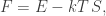 i.e. maximize the entropy
  subject to a constraint on the expected energy
We get the measure
Other observables about the spring’s path give conjugate variables whose product is energy. Given constraint on the average position of the spring at the halfway point, we get a conjugate force: pulling the spring out of equilibrium requires a force.
Statistical ensemble of thermometers with ensemble temperature T₂ [unitless].
We minimize the “free entropy” , i.e. we maximize the entropy
  subject to a constraint on the expected entropy lost
We get the measure
Given a constraint on the average position at the halfway point, we get a conjugate inverse length that tells how much entropy is lost when the thermometer shrinks by
Statistical ensemble of functions q with ensemble temperature T₂ [Kelvins].
We minimize the free energy i.e. we maximize the entropy
  subject to a constraint on the expected energy
We get the measure
Again, a constraint on the position would give a conjugate force. It’s a little harder to see how here, but given a non-optimal function we have an extra energy cost due to inefficiency that’s analogous to the stretching potential energy when pulling a spring out of equilibrium.
Thermo to quantum via Wick rotation of Lagrange multiplier
We allow a complex-valued measure as you did in the article above. We pick a logarithm for each
  and assume they don’t go through zero as we vary them. We also choose an imaginary Lagrange multiplier.
Normalize so
Define quantropy
Minimize the free action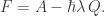
We get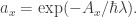 If
If  we get Feynman’s sum over histories. Surely something like the 2-slit experiment considers histories with a constraint on position at a particular time, and we get a conjugate momentum?
von Neumann Entropy However, this time we normalize so
Again allow complex-valued
Define von Neumann entropy
Allow quantum superposition of perturbed springs.
Allow quantum superpositions of thermometers.
 Get
Get  If
If  we get something like a sum over histories, but with a different normalization condition that converges because our set of paths is finite.
Allow quantum superposition of systems.
 Get
Get  If
If  we get the result of “Measure E, then heat the superposition T₁ degrees in a time much less than t seconds, then wait t seconds.” Different functions q in the superposition change the heat capacity differently and thus the systems end up at different energies.
So to sum up, there’s at least a three-way analogy between action, energy, and entropy depending on what you’re integrating over. You get a kind of “statics” if you extremize the integral by varying the path; by allowing multiple paths and constraints on observables, you get conjugate variables and “free” quantities that you want to minimize; and by taking the temperature to be imaginary, you get quantum systems.
I’ll make a little comment on this before I try hard to understand what you’re actually doing: your definition of ‘von Neumann entropy’ here looks wrong, or at least odd:
In quantum mechanics a mixed state—that is, a state in which we may have ignorance about the system—is described by a density matrix. This is a bounded linear operator on a Hilbert space that’s nonnegative and has
Here the trace is the sum of the diagonal entries in any orthonormal basis. The von Neumann entropy or simply entropy of such a mixed state is given by
We can find a basis in which is diagonal, and then
  is the probability of the mixed state being in the
  th pure state, and
is given in terms of these probabilities in a way that closely resembles classical entropy.
When is a pure state, the corresponding density matrix
  is the projection onto the vector
  , given by
If we diagonalize this we get a matrix with one 1 on the diagonal and the other entries zero. So, the von Neumann entropy of a pure state is zero! not something like
It makes sense that it’s zero, since we know as much as can be known about the system when it’s in a pure state!
On the other hand, if we take the pure state and ‘collapse’ it with respect to the standard basis of
  , we get a mixed state whose von Neumann entropy is
Three of your formulas do not parse (at least on my system).
Whoops, I forgot that LaTeX has a command \det but not a command \tr!
To get some intuition about quantropy we could try a ‘divide and conquer’ strategy. That means to investigate how quantropy of a ‘larger’ system comes from the quantropy of its ‘parts’. Without being precise of what ‘large’ and ‘part’ means at that point of the argument.
For entropy the situation is well-known. The entropy of two independent systems
  and
and  satisfies
Independence is crucial and the proof follows from the definition of entropy and observation that the combined system is in a state
  with probability
  where
where  (resp.
  ) denotes the probability that
  (resp.
  ) is in state
  (resp.
  ).
).
To derive a quantropy counterpart we remember that we are in a context of histories. Simply tensoring two systems does not seem adequate. We rather have to ‘glue’ them together. If we do this in an appropriate way (and my memory serves me well) the amplitude of a combined history then satisfies
Formally we can proceed as in the case of entropies to obtain
Thus we have encountered another entry in your analogy chart.
What I find remarkable is that the above equation of quantropy (contrary to the one for entropy) is indexed by histories. Thus one might be able to get some time evolution equation for quantropy (at least in the above case of independent histories) and thereby getting rid of your finiteness assumptions on .
.
Thanks for thinking about this stuff, Uwe!
My intuition tells me that quantropy should add both for ‘tensoring’ histories (i.e. setting two systems side by side and considering a history of the joint system made from a history of each part) and also for ‘composing’ histories (i.e. letting a system carry out a history for some interval of time and then another history after that).
My finiteness assumption on was mainly to sidestep the difficulties people always face with real-time path integrals (and secondarily to simplify the problem of choosing a branch for the logarithm when defining quantropy). I would like to try some examples where it’s not finite.
Gotta run!
[…] The table in John’s post on quantropy shows that energy and action are analogous […]
At the Universiti Putra Malaysia, Saeid Molladavoudi pointed me to this interesting paper, which claims to derive first the classical Hamilton–Jacobi equation and then Schrödinger’s equation from variational principles, where the action for the latter is obtained from the action for the former by adding a term proportional to a certain Fisher information:
• Marcel Reginatto, Derivation of the equations of nonrelativistic quantum
mechanics using the principle of minimum Fisher information.
I’ll have to check the calculations to see if they’re right! Then I can worry about what they actually mean, and if they’re related to the ‘principle of stationary quantropy’.
I found a paper that claims to give seemingly simple information theoretical derivation of QM from the uncertainty principle, maximum entropy distribution and Ehrenfest theorem:
http://vixra.org/abs/1912.0063
If that is correct, it would be nice to have a Newtonian approach to QM, along with Hamiltonian and Lagrangian.
Is that essentially just applying MaxEnt to the variance uncertainty?
It’s a sketchy introduction to Fourier transform pair of position-momentum and the use of maximum entropy is non-mathematical (if you compare to Ariel Caticha’s Entropic Dynamic that I have tried to read). But the treatment of the “inverse” Ehrenfest’s theorem is new to me. But apparently that watered-down entropy approach is not related to partition functions and quantropies.
Any way, the axiomatic framework of QM suggests that we are missing a fundamental principle that can be mixed with statistical mechanics. Maybe the concept of quantropy turns out to be fruitful.
That paper looks somewhat similar to another paper co-authored by Reginatto —which is the arxiv paper cited above. Click on reginatto and his paper with M Hall will show up (QM from UP).
the vixra paper cites reginatto (ref 2) —-i like that . i’m not in shape to try to go through these but the idea has been around along time—and even quantropy has. but its not like its common knowledge . stat mech, and QM and CM were always taught as opposites.
also i’m more philosopher or generalist than physicist so math isn’t easiest. i just haven’t found anyone interested in what these mean, only math to them. t.
[…] my post on quantropy I explained how the first three principles fit into a single framework if we treat Planck’s constant as an imaginary temperature […]
From Marco Frasca at The Gauge Connection on 1/25/2012:
Quantum mechanics and the square root of Brownian motion
John, an off-topic question. What LaTeX editor do you use in your blog? Any nice free alternative? My blog on Physics,Mathematics and more is to be launched soon. But I need suggestions on how to implement nice LaTeX code here.
Turning to your quantropy issue…The thermodynamics analogy can be something else. Indeed, the stuff related to entropic gravity, the rôle of entropy in General Relativity and the quantum/classical information theory strongly point out in that direction. Moreover, could , the Boltzmann’s constant, play some deeper fundamental aspect in the foundations of Quantum Physics than the own Planck’s constant? Recently, a group also suggests that Quantum Mechanics is “emergent”. The question I would ask next is…What are the most general entropy/quantropy functions/functionals that are mathematically and physically allowed? I just tend to think about Tsallis and non-extensive entropies as a big hint into the essential nature of entropy in the physical theories, maybe quantum gravity too whatever it is? A.Zeilinger himself told once than the key-word to understand QM and quantization itself was that information itself is quantized.
Latex math support is turned on by default for the free blogs on WordPress. http://en.support.wordpress.com/latex/
… and that’s what I use.
This is an interesting idea. I was thinking while I was reading it that it would be nice to have some kind of more intuitive understanding of what “quantropy” might be. One place to look for this might be Shannon’s information theory axioms.
There are three of these and they allow one to derive the functional form of entropy up to a multiplicative contant (or logarithm base). The meaty axiom is the second which just states that if one subdivides an outcome of a random variable into suboutcomes then the entropy increases by the new subsystem entropy weighted by the outcome probability. My intuitive view of this is that it relates entropy to coarse/fine graining which of course is central to what it means physically.
It might be interesting to start with Shannon’s axioms as applied to a “complex probability” i.e. quantum amplitude and see whether the functional form is essentially determined in the manner you are suggesting i.e. taking an appropriate branch of the complex logarithm. I started looking at Shannon’s original proof and it may need significant work to do this. You would also need to make some assumption about how a complex probability might work conditionally.
I wonder then if that works whether there is a relation between this axiom and the superposition princple in quantum mechanics….
Anyway enough idle speculation….
These are some sloppy thoughts towards a definition of quantropy based on your ideas so far. Under the assumption that quantropy is stationary we know that there are Lagrange multipliers such that
and thus
We plug these two equations into the formal definition of quantropy
and together with the constraint this yields
with
In the stationary situation can, at least formally, be interpreted as a zero-point quantropy. Albeit the zero-point (ground state) is not physical with its classicality 0 (
 ).
).
Let now be the classical action associated with a history
where is the mass of a particle and
  its potential energy. Feynman’s heuristic expression for the transition amplitude of the particle then is
It is tempting to define the transition amplitude of quantropy in the stationary situation as
for some suitable constants . This is not completely satisfactory from a foundational perspective, it might however be helpful in delivering some first examples. There are essentially two strategies to make sense of the above path integrals. One can apply the Trotter-Kato product formula or (due to Kac) do a Wick rotation and analytically extend a Wiener integral to the imaginary axis. Both ways are clustered with technicalities and thus, as a first approach, one could use a heuristic originally due to Feynman. He approximates continuous paths by polygonal paths with finitely many edges and uses a limit argument. As far as I can see one might approach some difficulties with the domain of the action that are not present in Feynman’s situation, however that seems to be more manageable than trying to define a logarithm of the amplitudes as requested in the formal definition of quantropy.
Uwe wrote:
Interesting that you say that: I’ve done a calculation like this, and I’ll present it in two blog posts here!
There are certainly lots of technical issues of mathematical rigor to consider. However, I think it’s even more important at this stage to get some physical intuition for quantropy. If Feynman had worried a lot about rigor we might never have gotten Feynman path integrals.
Excellent. I will certainly read this upcoming blog article.
In my first post in this series, we saw that rounding off a well-known analogy between statistical mechanics and quantum mechanics requires a new concept: ‘quantropy’. To get some feeling for this concept, we should look at some examples. But to do that, we need to develop some tools to compute quantropy. That’s what we’ll do today.
[…] Go check out John Baez on the remarkable analogies between statistical mechanics and quantum mechanics… and the idea of quantropy. […]
John, if you’d like to probe the depths of complex ignorance, I can help, or unhelp, depending on point of view.
Okay. I guess my main point is that I don’t see any difference between my ‘quantropy’ and your ‘entropy of a complex probability distribution’—except for words and perhaps motivation. As far as I can tell, they’re equal. I talk about finding a ‘critical point’ of quantropy given a constraint on the expected action, while you seem to talk about ‘maximizing complex ignorance’. I don’t know what it means to ‘maximize’ a complex-valued function; ‘critical point’ seems like the mathematically correct term here—but in terms of what you actually do, it seems to be the same thing I do.
But maybe I’m wrong. Can we throw out the words for a bit and focus on the math, and see what if any difference there is between our procedures?
Dear John. Maybe you and your readers could be interested in my post on Entropy in my blog. Comments, possible mistakes and suggestions are welcome:
John, , while I am primarily dealing with the probability distribution,
  , which I allow to be complex. You are inventing a new functional, quantropy,
  , while I am extremizing the usual entropy, or Ignorance,
  , extended for complex
  . One should raise an eyebrow at a complex probability. But under usual circumstances (a time independent Lagrangian), one gets
  for some amplitude,
  . The probabilities are real for observable outcomes. I’m not sure yet precisely how our two formulations are related, though they’re quite close. My formulation follows the principal of extremized entropy directly, while yours gives a more direct route to the amplitude, so I’m not sure which is better. I wonder if there’s a way to differentiate the two formulations as matching up with known physics or not.
There is an important difference, and not just with words. You are primarily dealing with the amplitude,
Garrett wrote:
As far as I can tell, a lot of these differences are just words. Let me use slightly different words to say the same thing:
I am primarily dealing with a complex-valued function satisfying
while you are primarily dealing with a complex-valued function satisfying
I am finding critical points of a function I call ‘quantropy’
while you are finding critical points of the function you call the ‘usual entropy extended for complex ‘:
‘:
These seem like suspiciously similar activities, no?
However, there seems to be some difference, because when I find my critical point, is not real-valued! So, maybe we’re finding critical points subject to different constraints, or something.
(By the way, I refuse to talk about ‘extremizing’ a complex-valued quantity, because ‘extremizing’ means ‘maximizing or minimizing’, and this is customarily used only for real-valued quantities. However the concept of ‘finding a critical point’—finding a place where the derivative of some quantity is zero—still makes sense for complex-valued quantities, and I believe that’s what you’re doing. But if you want to call this ‘extremizing’, I don’t really care too much, as long as I know what you’re doing.)
Heh. They are the same up to where you apparently stopped reading! But I’m calculating a probability, which happens to be equal to an amplitude times its conjugate under usual circumstances, . This is NOT the case for what you’re calculating, which is an amplitude,
  , that can be used to calculate probabilities. Maybe we call it criticalizing?
So, I guess I need to figure out what you’\re ‘criticizing’ (that’s my own jokey phrase for it), and what constraints you’re imposing, which gives an answer of the form
It seems we’re both criticizing the exact same thing:
where is a complex function on the set of paths constrained to have
But I’m imposing a further constraint on the expected action:
where is the action of a path. And, I’m considering solutions where the Lagrange multiplier for this constraint is
This does not give me a real answer for . It gives me the usual path integral prescription
where is a number chosen to ensure
  .
.
What assumptions are you using, to get real? I know, I should reread your paper!
I also impose the constraint , and obtain the same expression as you for
  . Since my
  is probability, this constraint has the physical interpretation of a universal action reservoir. This probability,
  , of a path is in general complex, but when we calculate a physical probability we find a real result. An example is the probability of a particle being seen at point
 at time
  . If the Lagrangian is time independent then the action of a path coming to this point from the past will be negative of the action of a path leaving this point into the future, so the probability factors into two multiplied parts,
  and its conjugate. In this way, the amplitude of paths from the past converging on
 at
at  is defined as
If you like, you can think of this as saying that the probability of seeing a particle at a point is the amplitude of paths coming to that point from the past times the amplitude of paths leaving that point into the future, which is the conjugate provided the dynamics is time reversible.
Ah, lovely, perhaps this will be more parsimonious:
Okay, thanks Garrett. I’m now convinced that you’re doing exactly what I’m doing, except:
1) you’re assuming the action of each path coming into a point from the past is the negative of the action of some path leaving this point into the future—or more precisely, the integral of the action over all paths going through that point is zero.
2) you’re using different words to describe what you’re doing,
3) you did it first.
Hmm, OK, but what I’d like to convince you of is that the probability, , is a different animal, and directly criticizing the complex ignorance is different then criticizing the quantropy. Also, I don’t need to assume that the probability factors as
  , but it’s nice that it does in usual cases. Also, it would be neat if someone could figure out the relationship between your path amplitude and my probability, and between the complex ignorance and quantropy, as I’m not sure precisely how they’re related.
That’s what I’m trying to figure out: how they’re related. So far it seems that mathematically they are identical except that at some point you impose the further assumption that ‘the action of a path coming to this point from the past will be negative of the action of a path leaving this point into the future’. This is why I’m trying to strip away the verbiage and look at just the math. I don’t always do that, but right now I’m trying to spot a mathematical difference, and I haven’t seen one.
That assumption is needed to show that, in that case, the probability can be written as the product of an amplitude and its conjugate. The probability derivation is fine without that assumption though.
I was reflecting this morning on what I think is the crux of the matter: “Why is the probability of a measured event equal to a squared quantum amplitude?” In the usual approach, one constructs or derives (as you do) the quantum amplitude, and then blithely squares it to get the probability. What I’ve tried to do is start with the fact that we’re dealing with a probability distribution, used MaxEnt to derive what it should be, and then show it’s the square of an amplitude. Although the two approaches are mathematically similar, I like being able to answer the question of why .
.
One tangible advantage of calling the numbers at issue “probabilities”, as opposed to “amplitudes”, may be that the former opens up the possibility of deriving the Born rule (as Garrett seems to do in the 2nd to last equation of his paper arXiv:physics/0605068v1), instead of having to postulate it.
Thanks Jim, that’s right. And it’s not just a difference of what we call things, but what we do with them. John needs to square his amplitude to get a probability, whereas my probability happens to factor into an amplitude squared.
Interesting…I suspect quantum mechanics and statistical mechanics has a deeper analogy besides the mathematical one..I wrote an article few years back: http://arxiv.org/abs/0712.1634
The idea: Quantum observables are analogous to Thermodynamic quantities
Hi There,
I don’t know if this article is still active (given its been almost a year). But, I found your analysis of quantropy quite interesting. It seems to have a context in Schwinger’s variational principle and the associated quantum effective action. For example, in a following post you express the quantropy exclusively in terms of where
where  is the partition function. Well, the quantum effective action is similarly expressed in terms of
  but as the Legendre transform wrt the external source field.
So, have you had a chance to look at the quantropy in the context of Schwinger’s variational principle and/or the quantum effective action (which relates to the Schwinger Dyson equations)? It seems these formulations are related.
Cheers,
Scott
I haven’t had a chance to look at quantropy since my last post here on the subject. But now that I’m back at U. C. Riverside accruing grad students, I’d like to write a paper on it… and your idea sounds very very helpful. I’m not familiar with Schwinger’s variational principle, but I’ve certainly seen quantum field theory calculations that use and take derivatives with respect to external source fields. So, I should expand my horizons a bit and connect this quantropy idea with those other ideas. They’re all part of a package of ideas that work both for quantum theory and statistical mechanics.
Good to hear that these ideas were not dead but only sleeping.
Very cool. Looking forward to learning more about this all! It’s really fascinating stuff.
I was thinking a bit more about all of this and had a couple additional thoughts:
1. Supposedly, Schwinger was motivated to formulate his variational principle ($latex \delta = i $ which describes the variation of the transition amplitude between the states $latex $ in terms of the classical action ) as the dynamical principle of quantum mechanics inspired by Feynmans path integral. Both Schwinger’s variational principle and Feynmans path integral can be used to derive Schrodingers equation, so they are alternate formulations of quantum mechanics that use the classical action. Bryce Dewitt advocated that infact Feynmans path integral is the
  of Schwinger’s variation (which itself was expressive of Peierl’s bracket). When I saw your derivation of Feynmans path integral from a stationary principle it reminded me of Schwinger’s variational principle because I know that that principle allows a sort of reconstruction of the path integral from the stationary principle. Hence the variation of the quantropy should somehow be related to Schwinger’s formulation. It doesn’t seem to be a trivial relation since the formulations though similar are quite different.
2. I was also reminded how in his ‘Statistical Physics’ text Feynman endorses the partition function and describes how in Stat Mech everything ‘builds up to or descends from it’. I suppose because the quantum path integral has its own partition function interpretation, similar arguments are applicable?
Very interesting stuff! Looking forward to thinking and learning more about all of this!
Cheers,
Scott
Sorry, having trouble with iPad. Should read for Schwinger’s variation
I was surprised to discover (or maybe rediscover, I’m not sure yet) that just as statistical mechanics is governed by the principle of maximum entropy, quantum mechanics is governed by a principle of maximum ‘quantropy’. The analogy between statistical mechanics and quantum mechanics has been known at least since Feynman and Schwinger. But this basic aspect was never explained to me!
If you have carefully read all my previous posts on quantropy (Part 1, Part 2 and Part 3), there’s only a little new stuff here. But still, it’s better organized […]
John wrote:
This blog post seems to suggest that next to this definition (which if I understand correctly is due to Boltzmann and Gibbs) there exists yet another definition of Gibbs entropy. But since the corresponding article is behind a paywall and there are no formulas given I may have interpreted wrongly.
Gibbs’ definition of entropy is essentially the same, though often with an integral instead of a sum, and often with a factor of Boltzmann’s constant in front:
• Entropy (statistical mechanics): Gibbs entropy formula, Wikipedia.
But in the blog post it is written that:
I don’t know how much one could trust this wikipedia article, like in the definition on the right side some terms seems to have vanished.
I don’t know what you mean by ‘some terms seem to have vanished’. The formula I see is fine:
You can find it in any decent textbook. It’s often called Boltzmann–Gibbs entropy. But this, and the fact that it permits negative temperatures, makes me realize that in the blog article you cite, Dunkel must be referring to some other definition of entropy when he talk about “Gibbs’ definition”:
We can read Dunkel and Hilbert’s paper for free here, and try to understand what they’re talking about:
• Dunkel and Hilbert, Consistent thermostatistics forbids negative absolute temperatures, Nature Physics (8 December 2013).
At least we can do so today: tomorrow it might be gone!
It turns out they are arguing in favor of a formula like this:
and against a formula like this:
Here is the number of states with energy
  , and
, and  is a mysterious quantity with dimensions of energy, chosen to make
dimensionless.
Both these formulas are variants of the microcanonical ensemble… which you can think of as a particular recipe for choosing the probabilities , if you like. But neither is the most common variant! I never use either of these formulas!
The amusing part to me is the mysterious quantity with dimensions of energy, chosen to make the argument of the logarithm dimensionless. This reminds me of what I’ve been talking about in Part 4 of this series! But it’s somewhat different.
I’m skimming this, and it seems to say this: The “Gibbs entropy” is defined as S_G = k_B log Omega where Omega is the grand total number of states… exactly what we all know and love as the formula for entropy. However, there is an alternate definition which seems to be very popular, as “most” (???) textbooks now advocate it, and “most”(???) researchers use it: it is S_B = k_B log epsilon (dOmega/dE) where dOmega/dE is the density of states and epsilon is a constant with dimension of energy (needed to make argument of the log dimensionless, of course). I can’t attest to the “most” part, but they do say this: “Hertz proved in 1910 that S_G is an adiabatic invariant21 . His work was highly commended by Planck22 and Einstein, who closes
his comment23 by stating that he would not have written some of his
papers had he been aware of Gibbs’ comprehensive treatise14 .”
So, historically, there has been confusion between S_G and S_B … yet they are essentially identical and equivalent for large, macroscopic, classical systems. (see below; its an off-by-one counting problem, for an N-particle system)
It turns out that if you plug these two into the standard textbook equations, you get two different definitions of a temperature. (call them T_G and T_B). You can measure T_B by using an ideal classical gas. If you couple the ideal classical gas to a quantum simple harmonic oscillator, you find that the T_B of the oscillator can be negative, when your thermometer is small enough… Whoops. By contrast, T_G stays positive.
Similarly, heat capacity stays positive if calculated from the S_G definition, and so on. The rest of the paper articulates and explores all the consequences of this.
So, anyway, my universe stands unshaken: I always use S_G. Its possible that S_B was in my textbooks too, I don’t recall.
BTW, later on, they state/show that T_B is the temperature of an N-particle system when you accidentally counted only up to (N-1). So it’s an off-by-one counting problem.
Ooops, sorry, I just noticed that I replied out-of-context; John already provides more or less the same answer.
John wrote:
I am sorry over the holidays I don’t check Azimuth as often as I did during the year, so I didn’t get your message in time. I was anyways mentioning the paper mostly because you mentioned negative temperatures earlier. So it seems there are many definitions of entropy.
typo:
negative
entropies->negative absolute temperaturesI prefer to say that Shannon-Boltzmann-Gibbs entropy is a single concept
that branches into many concepts depending on what measure space we use, what measure
  we use, and most importantly what probability distribution
  we use. Making different choices we get both
and
and also many other famous formulas.
But this is because I like to unify things. I don’t like having a bunch of unrelated concepts floating around in my brain: it hurts! I prefer to have a few general concepts and derive the rest as special cases.
In the box the state sum term (between line 2 and 3 in the formula) seems to have disappeared.
???
On a first glance at least it doesn’t look as if you get that entropies with the Boltzmann distribution and you wrote yourself that it is important for extremizing the free energy.
Moreover I am not sure about that but I could imagine that you could come up with a different integral than the Shannon one with which appropriate choices of measure and distribution could also lead to the Gibbs and Boltzmann entropies, but I might be wrong.
By the way: Who made it snowing on Azimuth?
Nad wrote:
Oh, I didn’t look at that box. I was only pointing you to the main explanation. If there’s a typo in that box, I’ll try to fix it.
I don’t know what you mean. I’m trying to tell you that the entropy of a probability distribution
is a single concept. This is the fundamental concept of entropy! This is what I meant by Shannon–Boltzmann–Gibbs entropy: all three guys contributed to our understanding of this concept.
When we maximize entropy subject to a constraint on
we get the Boltzmann distribution. Maximizing entropy subject to this constraint is also equivalent to minimizing free energy
for some value of But these are theorems about entropy, not different concepts of entropy!
It’s very cold here.
I find the snow pretty annoying. John, with your cape and your superpowers, can’t you make it stop?
As soon as it warms up a bit.
Nice analysis of the two entropy definitions here:
• E. T. Jaynes, Gibbs vs Boltzmann Entropies, Amer. J. Phys. 33 (1965), 391–398.
Thanks! And thanks to Nadja for pointing out these definitions on Wikipedia, where Boltzmann entropy is called ‘surface entropy’. It’s worth noting that Boltzmann entropy is invariant under and
and  , while Gibbs entropy is not: its definition breaks this symmetry, since it’s the logarithm of the measure of the set of states where the energy is less than some constant, instead of equal to it. This is undoubtedly why it treats negative temperatures differently than positive ones, as Dunkel and Hilbert are claiming. (They consider this a virtue; I’m unconvinced.)
I wrote below
Now “it looks” on Wikipedia, as if only more the volume entropy satisfies this condition, or may be I had overread something. Anyways thanks for pointing out the article it seems one might find more information on that issue in the article. It seems on afirst glance however that that what’s called Boltzmann and Gibbs entropies there is again different from what is mentioned in the Wikipedia article.
I wrote
with “that entropies” I meant the Gibbs and Boltzmann entropies. That is it doesn’t look to me on a first glance that given the Boltzmann distribution that there exists a measure such that the Shannon entropy yields the Gibbs and Boltzmann entropies, but as said – thats only a guess at a first glance.
Are you currently in Riverside?
Nad wrote:
The idea is that taking Shannon entropy of certain other natural probability distributions gives the Gibbs and Boltzmann entropies
where is the volume of the set of states with energy
The Boltzmann distribution is the so-called canonical distribution, meaning it maximizes entropy subject to a contraint on the expected value of energy. But to get the so-called Boltzmann entropy we instead take the Shannon entropy of the so-called microcanonical distribution, which maximizes entropy subject to a different constraint: we actually fix the energy to the specific sharp value
To get the so-called Gibbs entropy we use a distribution that maximizes entropy subject to yet another constraint: we require that the energy be less than or equal to a specific value
Maximizing entropy while fixing the energy to a specific sharp value is mathematically somewhat problematic, which we see in the need for an arbitrary quantity with dimensions of energy.
Often people instead require that the energy lie in some interval![[E - \delta, E + \delta],](https://s0.wp.com/latex.php?latex=%5BE+-+%5Cdelta%2C+E+%2B+%5Cdelta%5D%2C&bg=ffffff&fg=333333&s=0&c=20201002) but the answer still depends on the arbitrary choice of
but the answer still depends on the arbitrary choice of  As we let
  and normalize appropriately we get
Yes. It’s warm there. I meant it’s cold here in the blog.
By the way, I’m going to Erlangen on January 16th and staying until mid-May, except for some side-trips. That will seem quite cold to me at first, since I’m used to Riverside and Singapore!
John wrote:
What you said in the first quote sounded to me that you were certain that you can derive the Gibbs and Boltzmann entropies from the Shannon entropy via choosing a measure and distribution. Now it sounds that this is just an idea that it could be that way.
It sounds as if the cold keeps you from going into the wood and from stop working. Moreover you are close to your collaborators in England that seems also good workwise.
By the way it looks as if there are also snowstorms on wordpress.
Nad wrote:
Whew, communication can be very difficult! I didn’t mean it was ‘just an idea’. I claim it’s a correct idea!
I explained the idea to you yesterday. I told you which distributions to use to obtain the Gibbs and Boltzmann entropies from the Shannon entropy. I forgot to mention that you need to use these along with usual measure on phase space. There’s a formula for that measure here, but it doesn’t matter at all: just assume phase space is some measure space with an energy function
  on it.
I repeat, for your convenience (and somewhat rewritten):
All the necessary calculations should be in a book somewhere, but I don’t know such a book, so I just did the calculations myself. You can do them yourself and check my work. There are some subtleties you’ll run into if you try, which may make you worry. However, I explained the main ones.
I don’t have the time to do these calculations. I just wanted to take the opportunity to eventually quickly straighten out some things which I had never fully understood. But it seems this is messier than that it would allow for a quick better understanding.
So just to give you a view onto some things which irritate me here, in case you are interested: If I look at the wikipedia entry for the microcanonical distribution then first “it looks” as if only the what is called volume (surface) entropy satisfies some kind of condition which relates the differentials of energy and entropy. That is there is no remark that the Boltzmann entropy would satisfy a similar relation (which would be different from what you say). So I wonder about that.
Moreover “it looks” as if the Boltzmann entropy would be more a kind of uncertainty rather than an average uncertainty as is the case for the Shannon entropy. That is in particular I don’t see immediately that plugging the microcanonical distribution into the Shannon entropy one gets the Boltzmann entropy. But I might underestimate the strangeness of performing the integral over this limit case distribution. In particular “it looks” to me as if the Boltzmann factor seems to be of a different nature than a measure factor. But as said I just “looked” at it so chances are big that that glance onto things leaves a wrong image.
[…] Hamiltonian or quantum mechanical view of the conservation of energy within the system (see Baez's Azimuth blog for further insight). In basic terms, the second derivative with respect to time represents the […]
Nice read! I’ll have to mull it over better when I can digest the formulas a bit more (unfortunately, I’m an engineer turned computational physicist and I have some degree of intolerance to doing heavy analysis like this. I usually tend to just throw the numbers in and crunch them with the power of algorithms).
I’ve ended on this site pondering a similar analogy and problem. My starting point was the problem of “correlations” in the many-body wavefunction, which are a bane for DFT calculations. The gist of the problem is: you have two interacting electrons, say, in a potential. Their effective wavefunction will have a certain degree of correlation built in; namely, if I know the position of electron 1, I now have SOME more knowledge about electron 2, though not certainties, of course (it’s not full on entanglement after all). This lowers the Von Neumann entropy of the wavefunction, of course. What makes me think is how there really is a “tradeoff” at work here. If there is only ONE potential well, for example, the energy would be minimized by both electrons sitting into it. But of course there is repulsion among them, so in that situation the energy would be higher. So in order to lower it they sacrifice some of the entropy of the wavefunction. Of course no one says that if I were to express Schroedinger’s equation as a minimization principle analogous to the free energy one Von Neumann’s would be THE entropy that appears in it – it could just be a function which happens to be somewhat monotonous with the ‘true’ entropy. But looking at it, it should be possible to recast the time independent Schroedinger equation with your formalism if one performs a Wick rotation and calculates only the closed loops in the path integral.
Now of course I say all that but the thought of the math scares the hell out of me.
Thanks John.
Naive question: isn’t ‘h bar’ (reduced Planck constant) a constant by itself? What does limit of h bar tending to zero mean? What is the motivation?
If you take the equations of quantum mechanics and carefully take a limit where you get classical mechanics. If you take the equations of general relativity and take a limit where
  you get Newtonian gravity. If you take the equations of general relativity and take a limit where
  you get special relativity. So, limits of this sort are essential for understanding how more sophisticated theories of physics reduce to earlier theories.
It’s natural to ask what it means to take these limits, given that you can’t actually change the constants of nature. The answer lies in the fact that these aren’t dimensionless constants. It doesn’t make sense to ask what would happen as since
since  is dimensionless. But
  has units of action,
  has units of velocity, and
  has units of force times distance squared per mass squared.
So, if we’re studying a physics problem where all the velocities involved are small compared to the speed of light— is very small for all velocities
  in your problem—you typically can get a good approximate answer by taking the limit where
  And by changing units in a clever way, this can be reinterpreted as taking a limit where
  is held constant but
  The latter approach is often more convenient, because you just need to let one thing go to infinity (namely
  ) instead of letting lots of things go to infinity (all the velocities
  in your problem).
Similarly, in a physics problem where all the actions involved are large compared to classical mechanics is typically a good approximation to quantum mechanics. And it’s often convenient to study this by holding the actions that apprear in your problem constant but letting
In short, it involves a clever use of dimensional analysis.
[…] was some “recent” work by John Baez, which he described in his blog and also a paper. He also tried to make sense of Wick rotations by making use of it in a classical […]