Warming Slowdown? (Part 1)

1. How Heat Flows and Why It Matters

Is there something missing in the recent climate temperature record?

Heat is most often experienced as energy density, related to temperature. While technically temperature is only meaningful for a body in thermal equilibrium, temperature is the operational definition of heat content, both in daily life and as a scientific measurement, whether at a point or averaged. For the present discussion, it is taken as given that increasing atmospheric concentrations of carbon dioxide trap and re-radiate Earth blackbody radiation to its surface, resulting in a higher mean blackbody equilibration temperature for the planet, via radiative forcing [Ca2014a, Pi2012, Pi2011, Pe2006].

The question is, how does a given joule of energy travel? Once on Earth, does it remain in atmosphere? Warm the surface? Go into the oceans? And, especially,if it does go into the oceans, what is its residence time before released to atmosphere? These are important questions [Le2012a, Le2012b]. Because of the miscibility of energy, questions of residence time are very difficult to answer. A joule of energy can’t be tagged with a radioisotope like matter sometimes can. In practice, energy content is estimated as a constant plus the time integral of energy flux across a well-defined boundary using a baseline moment.

Variability is a key aspect of natural systems, whether biological or large scale geophysical systems such as Earth’s climate [Sm2009]. Variability is also a feature of statistical models used to describe behavior of natural systems, whether they be straightforward empirical models or models based upon ab initio physical calculations. Some of the variability in models captures the variability of the natural systems which they describe, but some variability is inherent in the mechanism of the models, an artificial variability which is not present in the phenomena they describe. No doubt, there is always some variability in natural phenomena which no model captures. This variability can be partitioned into parts, at the risk of specifying components which are not directly observable. Sometimes they can be inferred.

Models of planetary climate are both surprisingly robust and understood well enough that appreciable simplifications, such as setting aside fluid dynamism, are possible, without damaging their utility [Pi2012]. Thus, the general outline of what long term or asymptotic and global consequences arise when atmospheric carbon dioxide concentrations double or triple are known pretty well. More is known from the paleoclimate record.What is less certain are the dissipation and diffusion mechanisms for this excess energy and its behavior in time [Kr2014, Sh2014a, Sh2014b, Sa2011]. There is keen interest in these mechanisms because of the implications differing magnitudes have for regional climate forecasts and economies [Em2011, Sm2011, Le2010]. Moreover, there is a natural desire to obtain empirical confirmation of physical calculations, as difficult as that might be, and as subjective as judgments regarding quality of predictions might be [Sc2014, Be2013, Mu2013a, Mu2013b, Br2006, Co2013, Fy2013, Ha2013, Ha2014, Ka2013a, Sl2013, Tr2013, Mo2012, Sa2012, Ke2011a, Kh2008a, Kh2008b, Le2005, De1982].

Observed rates of surface temperatures in recent decades have shown a moderating slope compared with both long term statistical trends and climate model projections [En2014, Fy2014, Sc2014, Ta2013, Tr2013, Mu2013b, Fy2013, Fy2013s, Be2013]. It’s the purpose of this article to present this evidence, and report the research literature’s consensus on where the heat resulting from radiative forcing is going, as well as sketch some implications of that containment.

2. Tools of the Trade

I’m Jan Galkowski. I’m a statistician and signals engineer, with an undergraduate degree in Physics and a Masters in EE & Computer Science. I work for Akamai Technologies of Cambridge, MA, where I study time series of Internet activity and other data sources, doing data analysis primarily using spectral and Bayesian computational methods.

I am not a climate scientist, but am keenly interested in the mechanics of oceans, atmosphere, and climate disruption. I approach these problems from that of a statistician and physical dynamicist. Climate science is an avocation. While I have 32 years experience doing quantitative analysis, primarily in industry, I have found that the statistical and mathematical problems I encounter at Akamai have remarkable parallels to those in some geophysics, such as hydrology and assessments of sea level rise, as well as in some population biology. Thus, it pays to read their literature and understand their techniques. I also like to think that Akamai has something significant to contribute to this problem of mitigating forcings of climate change, such as enabling and supporting the ability of people to attend business and science meetings by high quality video call rather than hopping on CO₂-emitting vehicles.

As the great J. W. Tukey said:

The best thing about being a statistician is that you get to play in everyone’s backyard.

Anyone who doubts the fun of doing so, or how statistics enables such, should read Young.

3. On Surface Temperatures, Land and Ocean

Independently of climate change, monitoring surface temperatures globally is a useful geophysical project. They are accessible, can be measured in a number of ways, permit calibration and cross-checking, are taken at convenient boundaries between land-atmosphere or ocean-atmosphere, and coincide with the living space about which we most care. Nevertheless, like any large observational effort in the field, such measurements need careful assessment and processing before they can be properly interpreted. The Berkeley Earth Surface Temperature (“BEST”) Project represents the most comprehensive such effort, but it was not possible without many predecessors, such as HadCRUT4, and works by Kennedy, et al and Rohde [Ro2013a, Mo2012, Ke2011a, Ke2011b, Ro2013b].

Surface temperature is a manifestation of four interacting processes. First, there is warming of the surface by the atmosphere. Second, there is lateral heating by atmospheric convection and latent heat in water vapor. Third, during daytime, there is warming of the surface by the Sun or insolation which survives reflection. Last, there is warming of the surface from below, either latent heat stored subsurface, or geologic processes. Roughly speaking, these are ordered from most important to least. These are all manifestations of energy flows, a consequence of equalization of different contributions of energy to Earth.

Physically speaking, the total energy of the Earth climate system is a constant plus the time integral of energy of non-reflected insolation less the energy of the long wave radiation or blackbody radiation which passes from Earth out to space, plus geothermal energy ultimately due to radioisotope decay within Earth’s aesthenosphere and mantle, plus thermal energy generated by solid Earth and ocean tides, plus waste heat from anthropogenic combustion and power sources [Decay]. The amount of non-reflected insolation depends upon albedo, which itself slowly varies. The amount of long wave radiation leaving Earth for space depends upon the amount of water aloft, by amounts and types of greenhouse gases, and other factors. Our understanding of this has improved rapidly, as can be seen by contrasting Kiehl, et al in 1997 with Trenberth, et al in 2009 and the IPCC’s 2013 WG1 Report [Ki1997, Tr2009, IP2013]. Steve Easterbrook has given a nice summary of radiative forcing at his blog, as well as provided a succinct recap of the 2013 IPCC WG1 Report and its take on energy flows elsewhere at the The Azimuth blog. I refer the reader to those references for information about energy budgets, what we know about them, and what we do not.

Some ask whether or not there is a physical science basis for the “moderation” in global surface temperatures and, if there is, how that might work. It is an interesting question, for such a conclusion is predicated upon observed temperature series being calibrated and used correctly, and, further, upon insufficient precision in climate model predictions, whether simply perceived or actual. Hypothetically, it could be that the temperature models are not being used correctly and the models are correct, and which evidence we choose to believe depends upon our short-term goals. Surely, from a scientific perspective, what’s wanted is a reconciliation of both, and that is where many climate scientists invest their efforts. This is also an interesting question because it is, at its root, a statistical one, namely, how do we know which model is better [Ve2012, Sm2009, Sl2013, Ge1998, Co2006, Fe2011b, Bu2002]?

A first graph, Figure 1, depicting evidence of warming is, to me, quite remarkable. (You can click on this or any figure here, to enlarge it.)

$Ocean temperatures at depth$

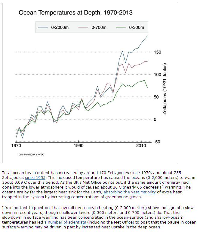
Figure 1. Ocean temperatures at depth, from Yale Climate Forum.

A similar graph is shown in the important series by Steve Easterbrook recapping the recent IPCC Report. A great deal of excess heat is going into the oceans. In fact, most of it is, and there is an especially significant amount going deep into the southern oceans, something which may have implications for Antarctica.

This can happen in many ways, but one dramatic way is due to a phase of the El Niño Southern Oscillation} (“ENSO”). Another way is storage by the Atlantic Meridional Overturning Circulation (“AMOC”) [Ko2014].

The trade winds along the Pacific equatorial region vary in strength. When they are weak, the phenomenon called El Niño is seen, affecting weather in the United States and in Asia. Evidence for El Niño includes elevated sea-surface temperatures (“SSTs”) in the eastern Pacific. This short-term climate variation brings increased rainfall to the southern United States and Peru, and drought to east Asia and Australia, often triggering large wildfires there.

The reverse phenomenon, La Niña, is produced by strong trades, and results in cold SSTs in the eastern Pacific, and plentiful rainfall in east Asia and northern Australia. Strong trades actually pile ocean water up against Asia, and these warmer-than-average waters push surface waters there down, creating a cycle of returning cold waters back to the eastern Pacific. This process is depicted in Figures 2 and 3. (Click to see a nice big animated version.)

Figure 2. Oblique view of variability of Pacific equatorial region from El Niño to La Niña and back. Vertical height of ocean is exaggerated to show piling up of waters in the Pacific warm pool.

Figure 3. Trade winds vary in strength, having consequences for pooling and flow of Pacific waters and sea surface temperatures.

At its peak, a La Niña causes waters to accumulate in the Pacific warm pool, and this results in surface heat being pushed into the deep ocean. To the degree to which heat goes into the deep ocean, it is not available in atmosphere. To the degree to which the trades do not pile waters into the Pacific warm pool and, ultimately, into the depths, that warm water is in contact with atmosphere [Me2011]. There are suggestions warm waters at depth rise to the surface [Me2013].

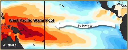
$Strong trade winds cause the warm surface waters of the equatorial Pacific to pile up against Asia$

Figure 4. Strong trade winds cause the warm surface waters of the equatorial Pacific to pile up against Asia.

Documentation of land and ocean surface temperatures is done in variety of ways. There are several important sources, including Berkeley Earth, NASA GISS, and the Hadley Centre/Climatic Research Unit (“CRU”) data sets [Ro2013a, Ha2010, Mo2012] The three, referenced here as BEST, GISS, and HadCRUT4, respectively, have been compared by Rohde. They differ in duration and extent of coverage, but allow comparable inferences. For example, a linear regression establishing a trend using July monthly average temperatures from 1880 to 2012 for Moscow from GISS and BEST agree that Moscow’s July 2010 heat was 3.67 standard deviations from the long term trend [GISS-BEST]. Nevertheless, there is an important difference between BEST and GISS, on the one hand, and HadCRUT4.

BEST and GISS attempt to capture and convey a single best estimate of temperatures on Earth’s surface, and attach an uncertainty measure to each number. Sometimes, because of absence of measurements or equipment failures, there are no measurements, and these are clearly marked in the series. HadCRUT4 is different. With HadCRUT4 the uncertainty in measurements is described by a hundred member ensemble of values, actually a 2592-by-1967 matrix. Rows correspond to observations from 2592 patches, 36 in latitude, and 72 in longitude, with which it represents the surface of Earth. Columns correspond to each month from January 1850 to November 2013. It is possible for any one of these cells to be coded as “missing”. This detail is important because HadCRUT4 is the basis for a paper suggesting the pause in global warming is structurally inconsistent with climate models. That paper will be discussed later.

4. Rumors of Pause

Figure 5 shows the global mean surface temperature anomalies relative to a standard baseline, 1950-1980. Before going on, consider that figure. Study it. What can you see in it?

$Global surface temperature anomalies relative to a 1950-1980 baseline$

Figure 5. Global surface temperature anomalies relative to a 1950-1980 baseline.

Figure 6 shows the same graph, but now with two trendlines obtained by applying a smoothing spline, one smoothing more than another. One of the two indicates an uninterrupted uptrend. The other shows a peak and a downtrend, along with wiggles around the other trendline. Note the smoothing algorithm is the same in both cases, differing only in the setting of a smoothing parameter. Which is correct? What is “correct”?

Figure 7 shows a time series of anomalies for Moscow, in Russia. Do these all show the same trends? These are difficult questions, but the changes seen in Figure 6 could be evidence of a warming “hiatus”. Note that, given Figure 6, whether or not there is a reduction in the rate of temperature increase depends upon the choice of a smoothing parameter. In a sense, that’s like having a major conclusion depend upon a choice of coordinate system, something we’ve collectively learned to suspect. We’ll have a more careful look at this in Section 5 next time. With that said, people have sought reasons and assessments of how important this phenomenon is. The answers have ranged from the conclusive “Global warming has stopped” to “Perhaps the slowdown is due to ‘natural variability”‘, to “Perhaps it’s all due to “natural variability” to “There is no statistically significant change”. Let’s see what some of the perspectives are.

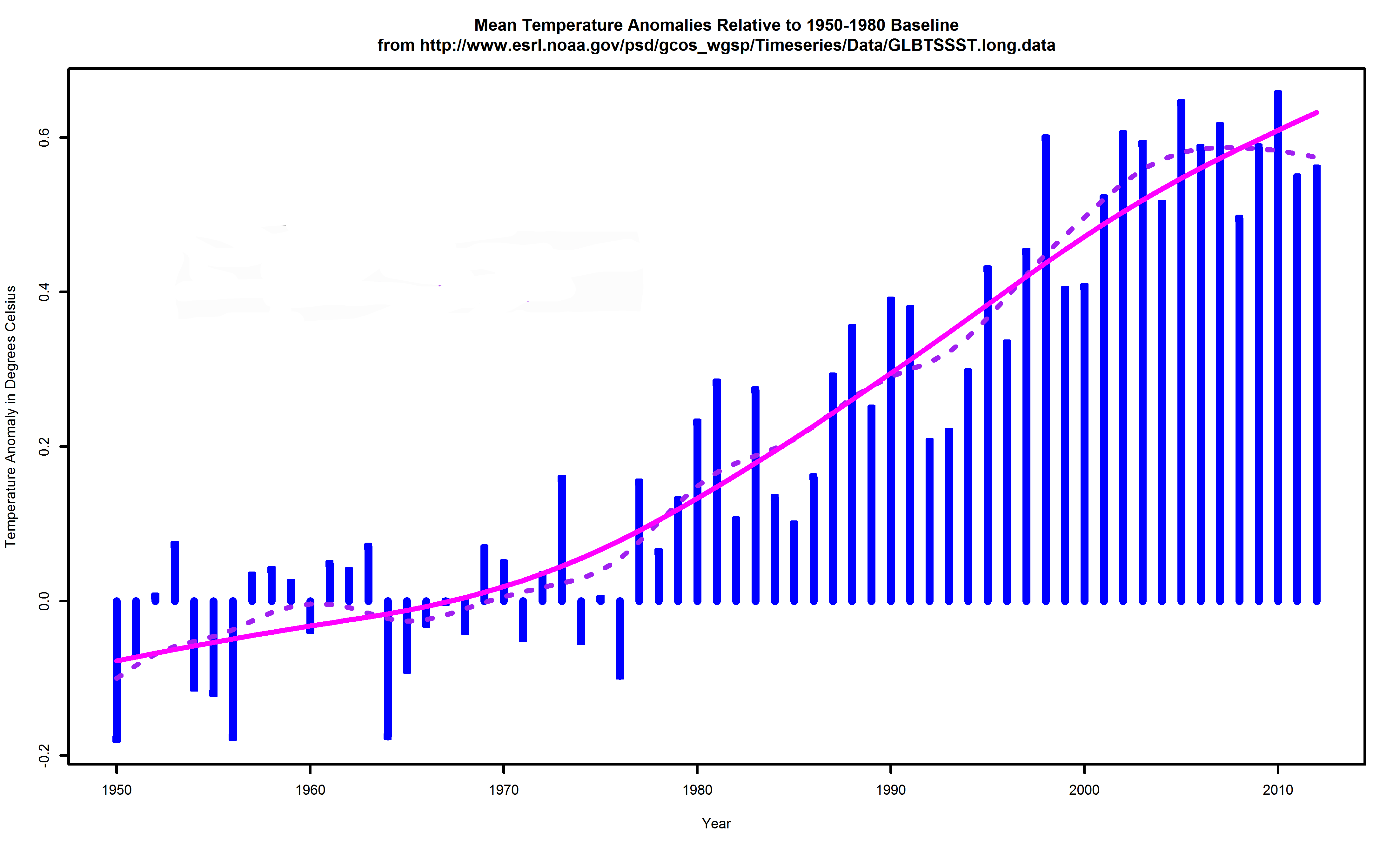
$Global surface temperature anomalies relative to a 1950-1980 baseline$

Figure 6. Global surface temperature anomalies relative to a 1950-1980 baseline, with two smoothing splines printed atop.

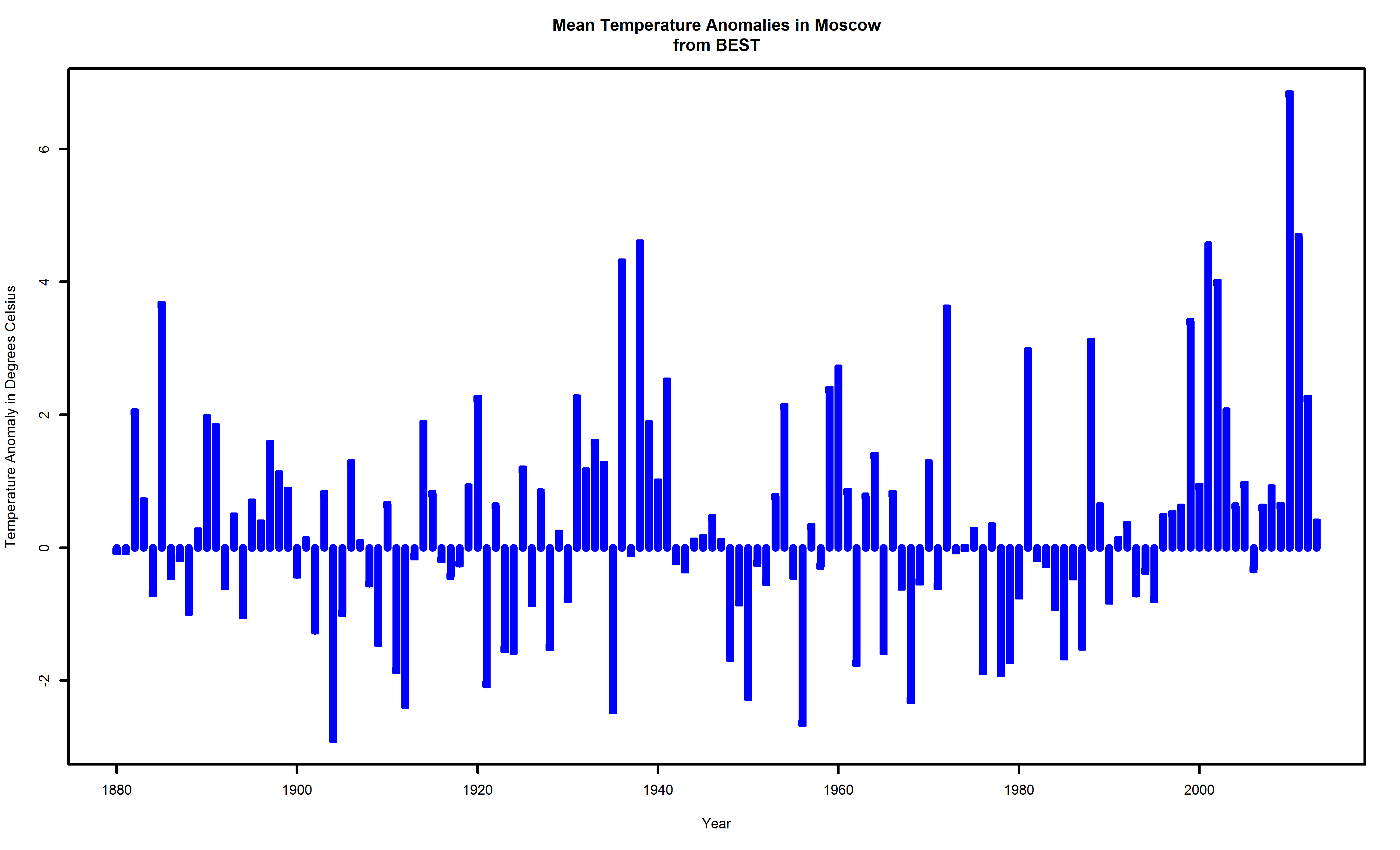
$Global surface temperature anomalies relative to a 1950-1980 baseline$

Figure 7. Temperature anomalies for Moscow, Russia.

It is hard to find a scientific paper which advances the proposal that climate might be or might have been cooling in recent history. The earliest I can find are repeated presentations by a single geologist in the proceedings of the Geological Society of America, a conference which, like many, gives papers limited peer review [Ea2000, Ea2000, Ea2001, Ea2005, Ea2006a, Ea2006b, Ea2007, Ea2008]. It is difficult to comment on this work since their full methods are not available for review. The content of the abstracts appear to ignore the possibility of lagged response in any physical system.

These claims were summarized by Easterling and Wehner in 2009, attributing claims of a “pause” to cherry-picking of sections of the temperature time series, such as 1998-2008, and what might be called media amplification. Further, technical inconsistencies within the scientific enterprise, perfectly normal in its deployment and management of new methods and devices for measurement, have been highlighted and abused to parlay claims of global cooling [Wi2007, Ra2006, Pi2006]. Based upon subsequent papers, climate science seemed to not only need to explain such variability, but also to provide a specific explanation for what could be seen as a recent moderation in the abrupt warming of the mid-late 1990s. When such explanations were provided, appealing to oceanic capture, as described in Section 3, the explanation seemed to be taken as an acknowledge of a need and problem, when often they were provided in good faith, as explanation and teaching [Me2011, Tr2013, En2014].

Other factors besides the overwhelming one of oceanic capture contribute as well. If there is a great deal of melting in the polar regions, this process captures heat from the oceans. Evaporation captures heat in water. No doubt these return, due to the water cycle and latent heat of water, but the point is there is much opportunity for transfer of radiative forcing and carrying it appreciable distances.

Note that, given the overall temperature anomaly series, such as Figure 6, and specific series, such as the one for Moscow in Figure 7, moderation in warming is not definitive. It is a statistical question, and, pretending for the moment we know nothing of geophysics, a difficult one. But there certainly is no any problem with accounting for the Earth’s energy budget overall, even if the distribution of energy over its surface cannot be specifically explained [Ki1997, Tr2009, Pi2012]. This is not a surprise, since the equipartition theorem of physics fails to apply to a system which has not achieved thermal equilibrium.

An interesting discrepancy is presented in a pair of papers in 2013 and 2014. The first, by Fyfe, Gillet, and Zwiers, has the (somewhat provocative) title “Overestimated global warming over the past 20 years”. (Supplemental material is also available and is important to understand their argument.) It has been followed by additional correspondence from Fyfe and Gillet (“Recent observed and simulated warming”) applying the same methods to argue that even with the Pacific surface temperature anomalies and explicitly accommodating the coverage bias in the HadCRUT4 dataset, as emphasized by Kosaka and Xie there remain discrepancies between the surface temperature record and climate model ensemble runs. In addition, Fyfe and Gillet dismiss the problems of coverage cited by Cowtan and Way, arguing they were making “like for life” comparisons which are robust given the dataset and the region examined with CMIP5 models.

How these scientific discussions present that challenge and its possible significance is a story of trends, of variability, and hopefully of what all these investigations are saying in common, including the important contribution of climate models.

Next Time

Next time I’ll talk about ways of estimating trends, what these have to say about global warming, and the work of Fyfe, Gillet, and Zwiers comparing climate models to HadCRUT4 temperature data.

Bibliography

Credentials. I have taken courses in geology from Binghamton University, but the rest of my knowledge of climate science is from reading the technical literature, principally publications from the American Geophysical Union and the American Meteorological Society, and self-teaching, from textbooks like Pierrehumbert. I seek to find ways where my different perspective on things canhelp advance and explain the climate science enterprise. I also apply my skills to working local environmental problems, ranging from inferring people’s use of energy in local municipalities, as well as studying things like trends in solid waste production at the same scales using Bayesian inversions. I am fortunate that techniques used in my professional work and those in these problems overlap so much. I am a member of the American Statistical Association, the American Geophysical Union, the American Meteorological Association, the International Society for Bayesian Analysis, as well as the IEEE and its signal processing society.
[Yo2014] D. S. Young, “Bond. James Bond. A statistical look at cinema’s most famous spy”, CHANCE Magazine, 27(2), 2014, 21-27, http://chance.amstat.org/2014/04/james-bond/.
[Ca2014a] S. Carson, Science of Doom, a website devoted to atmospheric radiation physics and forcings, last accessed 7 February 2014.
[Pi2012] R. T. Pierrehumbert, Principles of Planetary Climate, Cambridge University Press, 2010, reprinted 2012.
[Pi2011] R. T. Pierrehumbert, “Infrared radiative and planetary temperature”, Physics Today, January 2011, 33-38.
[Pe2006] G. W. Petty, A First Course in Atmospheric Radiation, 2^nd edition, Sundog Publishing, 2006.
[Le2012a] S. Levitus, J. I. Antonov, T. P. Boyer, O. K. Baranova, H. E. Garcia, R. A. Locarnini, A. V. Mishonov, J. R. Reagan, D. Seidov, E. S. Yarosh, and M. M. Zweng, “World ocean heat content and thermosteric sea level change (0-2000 m), 1955-2010”, Geophysical Research Letters, 39, L10603, 2012, http://dx.doi.org/10.1029/2012GL051106.
[Le2012b] S. Levitus, J. I. Antonov, T. P. Boyer, O. K. Baranova, H. E. Garcia, R. A. Locarnini, A. V. Mishonov, J. R. Reagan, D. Seidov, E. S. Yarosh, and M. M. Zweng, “World ocean heat content and thermosteric sea level change (0-2000 m), 1955-2010: supplementary information”, Geophysical Research Letters, 39, L10603, 2012, http://onlinelibrary.wiley.com/doi/10.1029/2012GL051106/suppinfo.
[Sm2009] R. L. Smith, C. Tebaldi, D. Nychka, L. O. Mearns, “Bayesian modeling of uncertainty in ensembles of climate models”, Journal of the American Statistical Association, 104(485), March 2009.
Nomenclature. The nomenclature can be confusing. With respect to observations, variability arising due to choice of method is sometimes called structural uncertainty [Mo2012, Th2005].
[Kr2014] J. P. Krasting, J. P. Dunne, E. Shevliakova, R. J. Stouffer (2014), “Trajectory sensitivity of the transient climate response to cumulative carbon emissions”, Geophysical Research Letters, 41, 2014, http://dx.doi.org/10.1002/2013GL059141.
[Sh2014a] D. T. Shindell, “Inhomogeneous forcing and transient climate sensitivity”, Nature Climate Change, 4, 2014, 274-277, http://dx.doi.org/10.1038/nclimate2136.
[Sh2014b] D. T. Shindell, “Shindell: On constraining the Transient Climate Response”, RealClimate, http://www.realclimate.org/index.php?p=17134, 8 April 2014.
[Sa2011] B. M. Sanderson, B. C. O’Neill, J. T. Kiehl, G. A. Meehl, R. Knutti, W. M. Washington, “The response of the climate system to very high greenhouse gas emission scenarios”, Environmental Research Letters, 6, 2011, 034005,
http://dx.doi.org/10.1088/1748-9326/6/3/034005.
[Em2011] K. Emanuel, “Global warming effects on U.S. hurricane damage”, Weather, Climate, and Society, 3, 2011, 261-268, http://dx.doi.org/10.1175/WCAS-D-11-00007.1.
[Sm2011] L. A. Smith, N. Stern, “Uncertainty in science and its role in climate policy”, Philosophical Transactions of the Royal Society A, 269, 2011 369, 1-24, http://dx.doi.org/10.1098/rsta.2011.0149.
[Le2010] M. C. Lemos, R. B. Rood, “Climate projections and their impact on policy and practice”, WIREs Climate Change, 1, September/October 2010, http://dx.doi.org/10.1002/wcc.71.
[Sc2014] G. A. Schmidt, D. T. Shindell, K. Tsigaridis, “Reconciling warming trends”, Nature Geoscience, 7, 2014, 158-160, http://dx.doi.org/10.1038/ngeo2105.
[Be2013] “Examining the recent “pause” in global warming”, Berkeley Earth Memo, 2013, http://static.berkeleyearth.org/memos/examining-the-pause.pdf.
[Mu2013a] R. A. Muller, J. Curry, D. Groom, R. Jacobsen, S. Perlmutter, R. Rohde, A. Rosenfeld, C. Wickham, J. Wurtele, “Decadal variations in the global atmospheric land temperatures”, Journal of Geophysical Research: Atmospheres, 118 (11), 2013, 5280-5286, http://dx.doi.org/10.1002/jgrd.50458.
[Mu2013b] R. Muller, “Has global warming stopped?”, Berkeley Earth Memo, September 2013, http://static.berkeleyearth.org/memos/has-global-warming-stopped.pdf.
[Br2006] P. Brohan, J. Kennedy, I. Harris, S. Tett, P. D. Jones, “Uncertainty estimates in regional and global observed temperature changes: A new data set from 1850”, Journal of Geophysical Research—Atmospheres, 111(D12), 27 June 2006, http://dx.doi.org/10.1029/2005JD006548.
[Co2013] K. Cowtan, R. G. Way, “Coverage bias in the HadCRUT4 temperature series and its impact on recent temperature trends”, Quarterly Journal of the Royal Meteorological Society, 2013, http://dx.doi.org/10.1002/qj.2297.
[Fy2013] J. C. Fyfe, N. P. Gillett, F. W. Zwiers, “Overestimated global warming over the past 20 years”, Nature Climate Change, 3, September 2013, 767-769, and online at http://dx.doi.org/10.1038/nclimate1972.
[Ha2013] E. Hawkins, “Comparing global temperature observations and simulations, again”, Climate Lab Book, http://www.climate-lab-book.ac.uk/2013/comparing-observations-and-simulations-again/, 28 May 2013.
[Ha2014] A. Hannart, A. Ribes, P. Naveau, “Optimal fingerprinting under multiple sources of uncertainty”, Geophysical Research Letters, 41, 2014, 1261-1268, http://dx.doi.org/10.1002/2013GL058653.
[Ka2013a] R. W. Katz, P. F. Craigmile, P. Guttorp, M. Haran, Bruno Sansó, M.L. Stein, “Uncertainty analysis in climate change assessments”, Nature Climate Change, 3, September 2013, 769-771 (“Commentary”).
[Sl2013] J. Slingo, “Statistical models and the global temperature record”, Met Office, May 2013, http://www.metoffice.gov.uk/media/pdf/2/3/Statistical_Models_Climate_Change_May_2013.pdf.
[Tr2013] K. Trenberth, J. Fasullo, “An apparent hiatus in global warming?”, Earth’s Future, 2013,
http://dx.doi.org/10.1002/2013EF000165.
[Mo2012] C. P. Morice, J. J. Kennedy, N. A. Rayner, P. D. Jones, “Quantifying uncertainties in global and regional temperature change using an ensemble of observational estimates: The HadCRUT4 data set”, Journal of Geophysical Research, 117, 2012, http://dx.doi.org/10.1029/2011JD017187. See also http://www.metoffice.gov.uk/hadobs/hadcrut4/data/current/download.html where the 100 ensembles can be found.
[Sa2012] B. D. Santer, J. F. Painter, C. A. Mears, C. Doutriaux, P. Caldwell, J. M. Arblaster, P. J. Cameron-Smith, N. P. Gillett, P. J. Gleckler, J. Lanzante, J. Perlwitz, S. Solomon, P. A. Stott, K. E. Taylor, L. Terray, P. W. Thorne, M. F. Wehner, F. J. Wentz, T. M. L. Wigley, L. J. Wilcox, C.-Z. Zou, “Identifying human infuences on atmospheric temperature”, Proceedings of the National Academy of Sciences, 29 November 2012, http://dx.doi.org/10.1073/pnas.1210514109.
[Ke2011a] J. J. Kennedy, N. A. Rayner, R. O. Smith, D. E. Parker, M. Saunby, “Reassessing biases and other uncertainties in sea-surface temperature observations measured in situ since 1850, part 1: measurement and sampling uncertainties”, Journal of Geophysical Research: Atmospheres (1984-2012), 116(D14), 27 July 2011, http://dx.doi.org/10.1029/2010JD015218.
[Kh2008a] S. Kharin, “Statistical concepts in climate research: Some misuses of statistics in climatology”, Banff Summer School, 2008, part 1 of 3. Slide 7, “Climatology is a one-experiment science. There is basically one observational record in climate”, http://www.atmosp.physics.utoronto.ca/C-SPARC/ss08/lectures/Kharin-lecture1.pdf.
[Kh2008b] S. Kharin, “Climate Change Detection and Attribution: Bayesian view”, Banff Summer School, 2008, part 3 of 3, http://www.atmosp.physics.utoronto.ca/C-SPARC/ss08/lectures/Kharin-lecture3.pdf.
[Le2005] T. C. K. Lee, F. W. Zwiers, G. C. Hegerl, X. Zhang, M. Tsao, “A Bayesian climate change detection and attribution assessment”, Journal of Climate, 18, 2005, 2429-2440.
[De1982] M. H. DeGroot, S. Fienberg, “The comparison and evaluation of forecasters”, The Statistician, 32(1-2), 1983, 12-22.
[Ro2013a] R. Rohde, R. A. Muller, R. Jacobsen, E. Muller, S. Perlmutter, A. Rosenfeld, J. Wurtele, D. Groom, C. Wickham, “A new estimate of the average Earth surface land temperature spanning 1753 to 2011”, Geoinformatics & Geostatistics: An Overview, 1(1), 2013, http://dx.doi.org/10.4172/2327-4581.1000101.
[Ke2011b] J. J. Kennedy, N. A. Rayner, R. O. Smith, D. E. Parker, M. Saunby, “Reassessing biases and other uncertainties in sea-surface temperature observations measured in situ since 1850, part 2: Biases and homogenization”, Journal of Geophysical Research: Atmospheres (1984-2012), 116(D14), 27 July 2011, http://dx.doi.org/10.1029/2010JD015220.
[Ro2013b] R. Rohde, “Comparison of Berkeley Earth, NASA GISS, and Hadley CRU averaging techniques on ideal synthetic data”, Berkeley Earth Memo, January 2013, http://static.berkeleyearth.org/memos/robert-rohde-memo.pdf.
[En2014] M. H. England, S. McGregor, P. Spence, G. A. Meehl, A. Timmermann, W. Cai, A. S. Gupta, M. J. McPhaden, A. Purich, A. Santoso, “Recent intensification of wind-driven circulation in the Pacific and the ongoing warming hiatus”, Nature Climate Change, 4, 2014, 222-227, http://dx.doi.org/10.1038/nclimate2106. See also http://www.realclimate.org/index.php/archives/2014/02/going-with-the-wind/.
[Fy2014] J. C. Fyfe, N. P. Gillett, “Recent observed and simulated warming”, Nature Climate Change, 4, March 2014, 150-151, http://dx.doi.org/10.1038/nclimate2111.
[Ta2013] Tamino, “el Niño and the Non-Spherical Cow”, Open Mind blog, http://tamino.wordpress.com/2013/09/02/el-nino-and-the-non-spherical-cow/, 2 September 2013.
[Fy2013s] Supplement to J. C. Fyfe, N. P. Gillett, F. W. Zwiers, “Overestimated global warming over the past 20 years”, Nature Climate Change, 3, September 2013, online at http://www.nature.com/nclimate/journal/v3/n9/extref/nclimate1972-s1.pdf.
Ionizing. There are tiny amounts of heating due to impinging ionizing radiation from space, and changes in Earth’s magnetic field.
[Ki1997] J. T. Kiehl, K. E. Trenberth, “Earth’s annual global mean energy budget”, Bulletin of the American Meteorological Society, 78(2), 1997, http://dx.doi.org/10.1175/1520-0477(1997)0782.0.CO;2.
[Tr2009] K. Trenberth, J. Fasullo, J. T. Kiehl, “Earth’s global energy budget”, Bulletin of the American Meteorological Society, 90, 2009, 311–323, http://dx.doi.org/10.1175/2008BAMS2634.1.
[IP2013] IPCC, 2013: Climate Change 2013: The Physical Science Basis. Contribution of Working Group I to the Fifth Assessment Report of the Intergovernmental Panel on Climate Change [Stocker, T.F., D. Qin, G.-K. Plattner, M. Tignor, S.K. Allen, J. Boschung, A. Nauels, Y. Xia, V. Bex and P.M. Midgley (eds.)]. Cambridge University Press, Cambridge, United Kingdom and New York, NY, USA, 1535 pp. Also available online at https://www.ipcc.ch/report/ar5/wg1/.
[Ve2012] A. Vehtari, J. Ojanen, “A survey of Bayesian predictive methods for model assessment, selection and comparison”, Statistics Surveys, 6 (2012), 142-228, http://dx.doi.org/10.1214/12-SS102.
[Ge1998] J. Geweke, “Simulation Methods for Model Criticism and Robustness Analysis”, in Bayesian Statistics 6, J. M. Bernardo, J. O. Berger, A. P. Dawid and A. F. M. Smith (eds.), Oxford University Press, 1998.
[Co2006] P. Congdon, Bayesian Statistical Modelling, 2^nd edition, John Wiley & Sons, 2006.
[Fe2011b] D. Ferreira, J. Marshall, B. Rose, “Climate determinism revisited: Multiple equilibria in a complex climate model”, Journal of Climate, 24, 2011, 992-1012, http://dx.doi.org/10.1175/2010JCLI3580.1.
[Bu2002] K. P. Burnham, D. R. Anderson, Model Selection and Multimodel Inference, 2^nd edition, Springer-Verlag, 2002.
[Ea2014a] S. Easterbrook, “What Does the New IPCC Report Say About Climate Change? (Part 4): Most of the heat is going into the oceans”, 11 April 2014, at the Azimuth blog, https://johncarlosbaez.wordpress.com/2014/04/11/what-does-the-new-ipcc-report-say-about-climate-change-part-4/.
[Ko2014] Y. Kostov, K. C. Armour, and J. Marshall, “Impact of the Atlantic meridional overturning circulation on ocean heat storage and transient climate change”, Geophysical Research Letters, 41, 2014, 2108–2116, http://dx.doi.org/10.1002/2013GL058998.
[Me2011] G. A. Meehl, J. M. Arblaster, J. T. Fasullo, A. Hu.K. E. Trenberth, “Model-based evidence of deep-ocean heat uptake during surface-temperature hiatus periods”, Nature Climate Change, 1, 2011, 360–364, http://dx.doi.org/10.1038/nclimate1229.
[Me2013] G. A. Meehl, A. Hu, J. M. Arblaster, J. Fasullo, K. E. Trenberth, “Externally forced and internally generated decadal climate variability associated with the Interdecadal Pacific Oscillation”, Journal of Climate, 26, 2013, 7298–7310, http://dx.doi.org/10.1175/JCLI-D-12-00548.1.
[Ha2010] J. Hansen, R. Ruedy, M. Sato, and K. Lo, “Global surface temperature change”, Reviews of Geophysics, 48(RG4004), 2010, http://dx.doi.org/10.1029/2010RG000345.
[GISS-BEST] 3.667 (GISS) versus 3.670 (BEST).
Spar. The smoothing parameter is a constant which weights a penalty term proportional to the second directional derivative of the curve. The effect is that if a candidate spline is chosen which is very bumpy, this candidate is penalized and will only be chosen if the data demands it. There is more said about choice of such parameters in the caption of Figure 12.
[Ea2009] D. R. Easterling, M. F. Wehner, “Is the climate warming or cooling?”, Geophysical Research Letters, 36, L08706, 2009, http://dx.doi.org/10.1029/2009GL037810.
Hiatus. The term hiatus has a formal meaning in climate science, as described by the IPCC itself (Box TS.3).
[Ea2000] D. J. Easterbrook, D. J. Kovanen, “Cyclical oscillation of Mt. Baker glaciers in response to climatic changes and their correlation with periodic oceanographic changes in the northeast Pacific Ocean”, 32, 2000, Proceedings of the Geological Society of America, Abstracts with Program, page 17, http://myweb.wwu.edu/dbunny/pdfs/dje_abstracts.pdf, abstract reviewed 23 April 2014.
[Ea2001] D. J. Easterbrook, “The next 25 years: global warming or global cooling? Geologic and oceanographic evidence for cyclical climatic oscillations”, 33, 2001, Proceedings of the Geological Society of America, Abstracts with Program, page 253, http://myweb.wwu.edu/dbunny/pdfs/dje_abstracts.pdf, abstract reviewed 23 April 2014.
[Ea2005] D. J. Easterbrook, “Causes and effects of abrupt, global, climate changes and global warming”, Proceedings of the Geological Society of America, 37, 2005, Abstracts with Program, page 41, http://myweb.wwu.edu/dbunny/pdfs/dje_abstracts.pdf, abstract reviewed 23 April 2014.
[Ea2006a] D. J. Easterbrook, “The cause of global warming and predictions for the coming century”, Proceedings of the Geological Society of America, 38(7), Astracts with Programs, page 235, http://myweb.wwu.edu/dbunny/pdfs/dje_abstracts.pdf, abstract reviewed 23 April 2014.
[Ea2006b] D. J. Easterbrook, 2006b, “Causes of abrupt global climate changes and global warming predictions for the coming century”, Proceedings of the Geological Society of America, 38, 2006, Abstracts with Program, page 77, http://myweb.wwu.edu/dbunny/pdfs/dje_abstracts.pdf, abstract reviewed 23 April 2014.
[Ea2007] D. J. Easterbrook, “Geologic evidence of recurring climate cycles and their implications for the cause of global warming and climate changes in the coming century”, Proceedings of the Geological Society of America, 39(6), Abstracts with Programs, page 507, http://myweb.wwu.edu/dbunny/pdfs/dje_abstracts.pdf, abstract reviewed 23 April 2014.
[Ea2008] D. J. Easterbrook, “Correlation of climatic and solar variations over the past 500 years and predicting global climate changes from recurring climate cycles”, Proceedings of the International Geological Congress, 2008, Oslo, Norway.
[Wi2007] J. K. Willis, J. M. Lyman, G. C. Johnson, J. Gilson, “Correction to ‘Recent cooling of the upper ocean”‘, Geophysical Research Letters, 34, L16601, 2007, http://dx.doi.org/10.1029/2007GL030323.
[Ra2006] N. Rayner, P. Brohan, D. Parker, C. Folland, J. Kennedy, M. Vanicek, T. Ansell, S. Tett, “Improved analyses of changes and uncertainties in sea surface temperature measured in situ since the mid-nineteenth century: the HadSST2 dataset”, Journal of Climate, 19, 1 February 2006, http://dx.doi.org/10.1175/JCLI3637.1.
[Pi2006] R. Pielke, Sr, “The Lyman et al paper ‘Recent cooling in the upper ocean’ has been published”, blog entry, September 29, 2006, 8:09 AM, https://pielkeclimatesci.wordpress.com/2006/09/29/the-lyman-et-al-paper-recent-cooling-in-the-upper-ocean-has-been-published/, last accessed 24 April 2014.
[Ko2013] Y. Kosaka, S.-P. Xie, “Recent global-warming hiatus tied to equatorial Pacific surface cooling”, Nature, 501, 2013, 403–407, http://dx.doi.org/10.1038/nature12534.
[Ke1998] C. D. Keeling, “Rewards and penalties of monitoring the Earth”, Annual Review of Energy and the Environment, 23, 1998, 25–82, http://dx.doi.org/10.1146/annurev.energy.23.1.25.
[Wa1990] G. Wahba, Spline Models for Observational Data, Society for Industrial and Applied Mathematics (SIAM), 1990.
[Go1979] G. H. Golub, M. Heath, G. Wahba, “Generalized cross-validation as a method for choosing a good ridge parameter”, Technometrics, 21(2), May 1979, 215-223, http://www.stat.wisc.edu/~wahba/ftp1/oldie/golub.heath.wahba.pdf.
[Cr1979] P. Craven, G. Wahba, “Smoothing noisy data with spline functions: Estimating the correct degree of smoothing by the method of generalized cross-validation”, Numerische Mathematik, 31, 1979, 377-403, http://www.stat.wisc.edu/~wahba/ftp1/oldie/craven.wah.pdf.
[Sa2013] S. Särkkä, Bayesian Filtering and Smoothing, Cambridge University Press, 2013.
[Co2009] P. S. P. Cowpertwait, A. V. Metcalfe, Introductory Time Series With R, Springer, 2009.
[Ko2005] R. Koenker, Quantile Regression, Cambridge University Press, 2005.
[Du2012] J. Durbin, S. J. Koopman, Time Series Analysis by State Space Methods, Oxford University Press, 2012.
Process variance. Here, the process variance was taken here to be $\frac{1}{50}$ of the observations variance.
Probabilities. “In this Report, the following terms have been used to indicate the assessed likelihood of an outcome or a result: Virtually certain 99-100% probability, Very likely 90-100%, Likely 66-100%, About as likely as not 33-66$%, Unlikely 0-33%, Very unlikely 0-10%, Exceptionally unlikely 0-1%. Additional terms (Extremely likely: 95-100%, More likely than not 50-100%, and Extremely unlikely 0-5%) may also be used when appropriate. Assessed likelihood is typeset in italics, e.g., very likely (see Section 1.4 and Box TS.1 for more details).”
[Ki2013] E. Kintsch, “Researchers wary as DOE bids to build sixth U.S. climate model”, Science 341 (6151), 13 September 2013, page 1160, http://dx.doi.org/10.1126/science.341.6151.1160.
Inez Fung. “It’s great there’s a new initiative,” says modeler Inez Fung of DOE’s Lawrence Berkeley National Laboratory and the University of California, Berkeley. “But all the modeling efforts are very short-handed. More brains working on one set of code would be better than working separately””.
Exchangeability. Exchangeability is a weaker assumption than independence. Random variables are exchangeable if their joint distribution only depends upon the set of variables, and not their order [Di1977, Di1988, Ro2013c]. Note the caution in Coolen.
[Di1977] P. Diaconis, “Finite forms of de Finetti’s theorem on exchangeability”, Synthese, 36, 1977, 271-281.
[Di1988] P. Diaconis, “Recent progress on de Finetti’s notions of exchangeability”, Bayesian Statistics, 3, 1988, 111-125.
[Ro2013c] J.C. Rougier, M. Goldstein, L. House, “Second-order exchangeability analysis for multi-model ensembles”, Journal of the American Statistical Association, 108, 2013, 852-863, http://dx.doi.org/10.1080/01621459.2013.802963.
[Co2005] F. P. A. Coolen, “On nonparametric predictive inference and objective Bayesianism”, Journal of Logic, Language and Information, 15, 2006, 21-47, http://dx.doi.org/10.1007/s10849-005-9005-7. (“Generally, though, both for frequentist and Bayesian approaches, statisticians are often happy to assume exchangeability at the prior stage. Once data are used in combination with model assumptions, exchangeability no longer holds ‘post-data’ due to the influence of modelling assumptions, which effectively are based on mostly subjective input added to the information from the data.”).
[Ch2008] M. R. Chernick, Bootstrap Methods: A Guide for Practitioners and Researches, 2^nd edition, 2008, John Wiley & Sons.
[Da2009] A. C. Davison, D. V. Hinkley, Bootstrap Methods and their Application, first published 1997, 11^th printing, 2009, Cambridge University Press.
[Mu2007] M. Mudelsee, M. Alkio, “Quantifying effects in two-sample environmental experiments using bootstrap condidence intervals”, Environmental Modelling and Software, 22, 2007, 84-96, http://dx.doi.org/10.1016/j.envsoft.2005.12.001.
[Wi2011] D. S. Wilks, Statistical Methods in the Atmospheric Sciences, 3^rd edition, 2011, Academic Press.
[Pa2006] T. N. Palmer, R. Buizza, R. Hagedon, A. Lawrence, M. Leutbecher, L. Smith, “Ensemble prediction: A pedagogical perspective”, ECMWF Newsletter, 106, 2006, 10–17.
[To2001] Z. Toth, Y. Zhu, T. Marchok, “The use of ensembles to identify forecasts with small and large uncertainty”, Weather and Forecasting, 16, 2001, 463–477, http://dx.doi.org/10.1175/1520-0434(2001)0162.0.CO;2.
[Le2013a] L. A. Lee, K. J. Pringle, C. I. Reddington, G. W. Mann, P. Stier, D. V. Spracklen, J. R. Pierce, K. S. Carslaw, “The magnitude and causes of uncertainty in global model simulations of cloud condensation nuclei”, Atmospheric Chemistry and Physics Discussion, 13, 2013, 6295-6378, http://www.atmos-chem-phys.net/13/9375/2013/acp-13-9375-2013.pdf.
[Gl2011] D. M. Glover, W. J. Jenkins, S. C. Doney, Modeling Methods for Marine Science, Cambridge University Press, 2011.
[Ki2014] E. Kintisch, “Climate outsider finds missing global warming”, Science, 344 (6182), 25 April 2014, page 348, http://dx.doi.org/10.1126/science.344.6182.348.
[GL2011] D. M. Glover, W. J. Jenkins, S. C. Doney, Modeling Methods for Marine Science, Cambridge University Press, 2011, Chapter 7.
[Le2013b] L. A. Lee, “Uncertainties in climate models: Living with uncertainty in an uncertain world”, Significance, 10(5), October 2013, 34-39, http://dx.doi.org/10.1111/j.1740-9713.2013.00697.x.
[Ur2014] N. M. Urban, P. B. Holden, N. R. Edwards, R. L. Sriver, K. Keller, “Historical and future learning about climate sensitivity”, Geophysical Research Letters, 41, http://dx.doi.org/10.1002/2014GL059484.
[Th2005] P. W. Thorne, D. E. Parker, J. R. Christy, C. A. Mears, “Uncertainties in climate trends: Lessons from upper-air temperature records”, Bulletin of the American Meteorological Society, 86, 2005, 1437-1442, http://dx.doi.org/10.1175/BAMS-86-10-1437.
[Fr2008] C. Fraley, A. E. Raftery, T. Gneiting, “Calibrating multimodel forecast ensembles with exchangeable and missing members using Bayesian model averaging”, Monthly Weather Review. 138, January 2010, http://dx.doi.org/10.1175/2009MWR3046.1.
[Ow2001] A. B. Owen, Empirical Likelihood, Chapman & Hall/CRC, 2001.
[Al2012] M. Aldrin, M. Holden, P. Guttorp, R. B. Skeie, G. Myhre, T. K. Berntsen, “Bayesian estimation of climate sensitivity based on a simple climate model fitted to observations of hemispheric temperatures and global ocean heat content”, Environmentrics, 2012, 23, 253-257, http://dx.doi.org/10.1002/env.2140.
[AS2007] “ASA Statement on Climate Change”, American Statistical Association, ASA Board of Directors, adopted 30 November 2007, http://www.amstat.org/news/climatechange.cfm, last visited 13 September 2013.
[Be2008] L. M. Berliner, Y. Kim, “Bayesian design and analysis for superensemble-based climate forecasting”, Journal of Climate, 21, 1 May 2008, http://dx.doi.org/10.1175/2007JCLI1619.1.
[Fe2011a] X. Feng, T. DelSole, P. Houser, “Bootstrap estimated seasonal potential predictability of global temperature and precipitation”, Geophysical Research Letters, 38, L07702, 2011, http://dx.doi.org/10.1029/2010GL046511.
[Fr2013] P. Friedlingstein, M. Meinshausen, V. K. Arora, C. D. Jones, A. Anav, S. K. Liddicoat, R. Knutti, “Uncertainties in CMIP5 climate projections due to carbon cycle feedbacks”, Journal of Climate, 2013, http://dx.doi.org/10.1175/JCLI-D-12-00579.1.
[Ho2003] T. J. Hoar, R. F. Milliff, D. Nychka, C. K. Wikle, L. M. Berliner, “Winds from a Bayesian hierarchical model: Computations for atmosphere-ocean research”, Journal of Computational and Graphical Statistics, 12(4), 2003, 781-807, http://www.jstor.org/stable/1390978.
[Jo2013] V. E. Johnson, “Revised standards for statistical evidence”, Proceedings of the National Academy of Sciences, 11 November 2013, http://dx.doi.org/10.1073/pnas.1313476110, published online before print.
[Ka2013b] J. Karlsson, J., Svensson, “Consequences of poor representation of Arctic sea-ice albedo and cloud-radiation interactions in the CMIP5 model ensemble”, Geophysical Research Letters, 40, 2013, 4374-4379, http://dx.doi.org/10.1002/grl.50768.
[Kh2002] V. V. Kharin, F. W. Zwiers, “Climate predictions with multimodel ensembles”, Journal of Climate, 15, 1 April 2002, 793-799.
[Kr2011] J. K. Kruschke, Doing Bayesian Data Analysis: A Tutorial with R and BUGS, Academic Press, 2011.
[Li2008] X. R. Li, X.-B. Li, “Common fallacies in hypothesis testing”, Proceedings of the 11^th IEEE International Conference on Information Fusion, 2008, New Orleans, LA.
[Li2013] J.-L. F. Li, D. E. Waliser, G. Stephens, S. Lee, T. L’Ecuyer, S. Kato, N. Loeb, H.-Y. Ma, “Characterizing and understanding radiation budget biases in CMIP3/CMIP5 GCMs, contemporary GCM, and reanalysis”, Journal of Geophysical Research: Atmospheres, 118, 2013, 8166-8184, http://dx.doi.org/10.1002/jgrd.50378.
[Ma2013b] E. Maloney, S. Camargo, E. Chang, B. Colle, R. Fu, K. Geil, Q. Hu, x. Jiang, N. Johnson, K. Karnauskas, J. Kinter, B. Kirtman, S. Kumar, B. Langenbrunner, K. Lombardo, L. Long, A. Mariotti, J. Meyerson, K. Mo, D. Neelin, Z. Pan, R. Seager, Y. Serra, A. Seth, J. Sheffield, J. Stroeve, J. Thibeault, S. Xie, C. Wang, B. Wyman, and M. Zhao, “North American Climate in CMIP5 Experiments: Part III: Assessment of 21st Century Projections”, Journal of Climate, 2013, in press, http://dx.doi.org/10.1175/JCLI-D-13-00273.1.
[Mi2007] S.-K. Min, D. Simonis, A. Hense, “Probabilistic climate change predictions applying Bayesian model averaging”, Philosophical Transactions of the Royal Society, Series A, 365, 15 August 2007, http://dx.doi.org/10.1098/rsta.2007.2070.
[Ni2001] N. Nicholls, “The insignificance of significance testing”, Bulletin of the American Meteorological Society, 82, 2001, 971-986.
[Pe2008] G. Pennello, L. Thompson, “Experience with reviewing Bayesian medical device trials”, Journal of Biopharmaceutical Statistics, 18(1), 81-115).
[Pl2013] M. Plummer, “Just Another Gibbs Sampler”, JAGS, 2013. Plummer describes this in greater detail at “JAGS: A program for analysis of Bayesian graphical models using Gibbs sampling”, Proceedings of the 3^rd International Workshop on Distributed Statistical Computing (DSC 2003), 20-22 March 2003, Vienna. See also M. J. Denwood, [in review] “runjags: An R package providing interface utilities, parallel computing methods and additional distributions for MCMC models in JAGS”, Journal of Statistical Software, and http://cran.r-project.org/web/packages/runjags/. See also J. Kruschke, “Another reason to use JAGS instead of BUGS”, http://doingbayesiandataanalysis.blogspot.com/2012/12/another-reason-to-use-jags-instead-of.html, 21 December 2012.
[Po1994] D. N. Politis, J. P. Romano, “The Stationary Bootstrap”, Journal of the American Statistical Association, 89(428), 1994, 1303-1313, http://dx.doi.org/10.1080/01621459.1994.10476870.
[Sa2002] C.-E. Särndal, B. Swensson, J. Wretman, Model Assisted Survey Sampling, Springer, 1992.
[Ta2012] K. E. Taylor, R.J. Stouffer, G.A. Meehl, “An overview of CMIP5 and the experiment design”, Bulletin of the American Meteorological Society, 93, 2012, 485-498, http://dx.doi.org/10.1175/BAMS-D-11-00094.1.
[To2013] A. Toreti, P. Naveau, M. Zampieri, A. Schindler, E. Scoccimarro, E. Xoplaki, H. A. Dijkstra, S. Gualdi, J, Luterbacher, “Projections of global changes in precipitation extremes from CMIP5 models”, Geophysical Research Letters, 2013, http://dx.doi.org/10.1002/grl.50940.
[WC2013] World Climate Research Programme (WCRP), “CMIP5: Coupled Model Intercomparison Project”, http://cmip-pcmdi.llnl.gov/cmip5/, last visited 13 September 2013.
[We2011] M. B. Westover, K. D. Westover, M. T. Bianchi, “Significance testing as perverse probabilistic reasoning”, BMC Medicine, 9(20), 2011, http://www.biomedcentral.com/1741-7015/9/20.
[Zw2004] F. W. Zwiers, H. Von Storch, “On the role of statistics in climate research”, International Journal of Climatology, 24, 2004, 665-680.
[Ra2005] A. E. Raftery, T. Gneiting , F. Balabdaoui , M. Polakowski, “Using Bayesian model averaging to calibrate forecast ensembles”, Monthly Weather Review, 133, 1155–1174, http://dx.doi.org/10.1175/MWR2906.1.
[Ki2010] G. Kitagawa, Introduction to Time Series Modeling, Chapman & Hall/CRC, 2010.
[Hu2010] C. W. Hughes, S. D. P. Williams, “The color of sea level: Importance of spatial variations in spectral shape for assessing the significance of trends”, Journal of Geophysical Research, 115, C10048, 2010, http://dx.doi.org/10.1029/2010JC006102.

This entry was posted on Thursday, May 29th, 2014 at 1:00 am and is filed under climate. You can follow any responses to this entry through the RSS 2.0 feed. You can leave a response, or trackback from your own site.

91 Responses to Warming Slowdown? (Part 1)

Vanessa Schweizer says:

29 May, 2014 at 2:55 pm

This is an excellent post! I can’t wait to read Part 2!

Reply
- John Baez says:
  
  29 May, 2014 at 3:39 pm
  
  Great! By the way, if you know people who’d enjoy writing good blog posts on climate science, ecology, environmental issues or the like, please send them in my direction! I assume you know the sort of thing we like here.
  
  Reply
WebHubTelescope says:

30 May, 2014 at 6:54 am

On the chaos scale of 1 to 10, where does ENSO fit?

Reply
- John Baez says:
  
  30 May, 2014 at 8:53 am
  
  What’s the “chaos scale”?
  
  Reply
  - WebHubTelescope says:
    
    30 May, 2014 at 1:36 pm
    
    On a chaos scale, a value of 10 would be a time series that would be unpredictable and a behavior very sensitive to initial conditions
    
    A value of 1 would be a time series that only appears chaotic but actually follows a predictably deterministic outcome that is relatively insensitive to initial conditions.
    
    The latter behavior is exemplified by processes that follow the Mathieu equation.
    
    I think ENSO is closer to a 1 than a 10 based the ease of which one can match the historical time series with the strong boundary conditions supplied by forcing functions such as the atmospheric Quasiperiodic Biennial Oscillations (QBO).
    http://contextearth.com/2014/05/27/the-soim-differential-equation
    
    The QBO agitates the Mathieu modulated ocean and generates the sloshing dynamics observed.
    
    In essence, the Mathieu equation supplies enough of a nonlinear transfer function to obscure the underlying periodicity. To the unaided eye, the behavior of ENSO looks very similar to red noise, but once the waveform is deconstructed, the real modulation pops out.
    
    This is some insanely cool math that is right up your alley, John and Jan.
    
    BTW, very few people are working this angle. I started looking at it because the dynamics of ENSO looked very similar to the Bloch waves of solid state physics that I cut my teeth on. There you have a wave function of an electron interacting strongly with the periodic potential of a crystal lattice, giving rise to the complicated band structure observed. No one calls that chaotic even though it appears that way in passing.
    
    Paul Pukite
    
    Reply
    - hypergeometric says:
      
      30 May, 2014 at 1:52 pm
      
      Um, don’t know much about this literature, but, just looking at it, the Mathieu equation looks like a spring motion equation with a time dependent spring coefficient. Do you know the literature well enough to tell if the Mathieu equation captures physical features of the ocean here? For example, is there some identification or relationship between the frequency component of the spring coefficient and depth to which warm water goes in the Pacific?
      
      No doubt simple models have their place in this work. Indeed, the climate models Professor Ray Pierrehumbert uses in his Principles of Planetary Climate are just graphs on paper.
    - WebHubTelescope says:
      
      30 May, 2014 at 2:14 pm
      
      Actually this approach applying Mathieu equations is very commonly used to model sloshing behavior in liquid-filled tanks. This is a good article:
      
      • J. B. Frandsen, “Sloshing motions in excited tanks,” Journal of Computational Physics, vol. 196, no. 1, pp. 53–87, 2004.
      
      And there is this for an analogy:
      
      • Shivamoggi, Bhimsen K. “Vortex motion in superfluid 4He: effects of normal fluid flow.” The European Physical Journal B 86.6 (2013): 1-7.
      
      “… Mathieu’s equation describing the parametric ampliﬁcation of Kelvin waves by the friction force. Equation (52) reveals again that the friction term associated with α inﬂuences the vortex motion in a qualitative way.”
      
      My thinking is that the QBO is parametrically amplifying the ocean’s Kelvin waves in a similar manner, leading to ENSO. Remember that the physics and math do not change just because of the scale of the system.
      
      I haven’t gotten around to deriving the characteristic frequency from the volume parameters. The common criticism is that the Pacific ocean is too shallow for these equations to be valid, yet the sloshing behavior is clearly evident, especially when you look at Jan’s Figure 2 and 3.
    - hypergeometric says:
      
      30 May, 2014 at 2:38 pm
      
      So, this is not my field, but *my* understanding of the physical oceanography is that the normal linear kinds of oscillations don’t work for much of the oceans because of the dominating and surprising effects of rotation. These create structure and eddies. Indeed, Kelvin waves themselves are, I believe, manifestations of these terms. (See Pedlosky, Waves in the Ocean and Atmosphere: Introduction to Wave Dynamics, 2003, Lecture 13, “Channel modes and the Kelvin wave”.) However, they do work for the ENSO, located as it is on the equator. As Pedlosky describes (2003, Lecture 18),
      
      The equator is a special region dynamically, most obviously because there the vertical component of the Earth’s rotation vanishes. It turns out to be, in consequence, a region in which certain linear waves have unusually strong signals and are involved in some important atmospheric and oceanic phenomena such as the Quasi-Biennial Oscillation in the atmosphere and the El Niño (ENSO) phenomenon in the ocean (and atmosphere).
      
      Thus, I would expect that while the Mathieu characterization would help with these, it may not be that useful elsewhere. But, as I say, this is not my field.
    - Nathan Urban says:
      
      2 June, 2014 at 4:47 pm
      
      There has been debate in the literature as to whether ENSO is best viewed in a “nonlinear deterministic” (i.e. chaotic) or a “linear stochastic” framework. Some discussion may be found in Chekroun et al. (2011).
  - John Baez says:
    
    31 May, 2014 at 7:14 am
    
    If I were looking at simple models of El Niño, I would look at the Zebiak–Cane model and the delayed-action oscillator. We got as far as writing up explanations of them here:
    
    • ENSO, Azimuth Library.
    
    but I would love software that would run on a web browser and illustrate either of these models. This paper suggests that it could make a fun high school project:
    
    • Ian Boutle, Richard H. S. Taylor, and Rudolf A. Roemer, El Niño and the delayed action oscillator, American Journal of Physics 75 (2007), 15–24.
    
    Of course it’s great that WebHubTel is trying new, different ideas.
    
    Reply
    - WebHubTelescope says:
      
      1 June, 2014 at 1:23 am
      
      Yes, I had run across the approaches that had been applying Delayed Differential Equations (DDE) which you compare the delayed-action oscillator to. Sorry that I missed the Azimuth library entry in my initial research search! My bad.
      
      What is also interesting is the delayed Mathieu equation, which is a hybrid of the DDE and the non-linear Mathieu.
      
      The connection between the two is that a delay with a difference term is the discrete version of the differential operator. Of course the delay here is intended to be less fine than a differential term and is meant to simulate interference over longer time intervals. This would be a wave that bounces off a boundary and comes back to interfere, much like as in a delayed action oscillator.
      
      As an interesting aside, as I was playing around with the Eureqa software, I decided to add a delay operator to the mix. What Eureqa does is try to find patterns in the data corresponding to math constructs, and so it started adding delay terms. Lo and behold, the correlations quickly became surprisingly strong. But then I realized that the delay terms were being added to emulate the second derivative, which is what I was trying to find patterns in. Oops! Lesson is that be very careful when mixing continuous math with discrete interval math.
- hypergeometric says:
  
  30 May, 2014 at 1:30 pm
  
  Usually, when getting quantitative about it, *chaos* is described in terms of a “Lyaponuv coffieicent“. That is, there is no single characterization of a predicted state in terms of uncertainty in initial conditions, but a whole possible range of such behaviors. Here, $\lambda$ is the Lyaponuv coefficent, per $|\delta \mathbf{Z}(t)| \approx e^{\lambda t} |\delta \mathbf{Z}_{0}|$ . You can also have cascades like $|\delta \mathbf{Z}(t)| \approx e^{e^{\lambda t}} |\delta \mathbf{Z}_{0}|$ . Which do you mean?
  
  If considered a dynamical system like one modeled by a large set of coupled differential equations, ENSO is an oscillation in it. In the long run, it averages out. (To quote Dr Tyson from the upcoming Cosmos, “Watch the man, not the dog.”) To us, it may matter substantially, since our lifetimes are so short.
  
  Reply
John Baez says:

30 May, 2014 at 11:42 am

Here’s a graph put out by NASA showing surface temperature, volcanos, and some index of El Niño activity up to 2011:

(Which El Niño index are they using—the multivariate ENSO index?)

There seems to be correlation, though also moments of anticorrelation like around 1993. Has someone tried to use this correlation to create a graph of “El Niño-corrected” surface temperatures? Has someone tried to see what this graph says about the recent surface temperature increase slowdown?

And some say we’re due for an El Niño starting this autumn. I’ve heard some claim this will be the end of the surface temperature increase slowdown. Has anyone tried to project surface temperatures forward for the next few years taking El Niño projections into account?

The NASA website created in 2011 says:

Hansen et al. (2010) argued, in anticipation of the inevitable shift from the then beginning La Niña to the next El Niño, that “The 12-month running mean global temperature in 2010 has reached a new record level for the period of instrumental data. It is likely that the 12-month mean will begin to decline in the second half of 2010. The subsequent minimum in the 12-month running mean is likely to be in 2011-2012 and not as deep as the 2008 minimum. The next maximum, likely to be in 2012-2014, will probably bring a new record global temperature, because of the underlying warming trend.”

The heat content of the upper 300 m of the equatorial Pacific Ocean (Fig. 8) is useful data for anticipating the next El Niño, because it precedes the Niño index by two months, which in turn precedes global temperature by four months. The data in Fig. 8, and data for the entire past century, also indicate that the El Niño cycle, although notorious variable, seldom goes straight from a deep La Niña into a strong El Niño. More commonly there is a build up over a few years. Thus, although the ocean heat content increased in the first half of 2011, reaching a positive anomaly level in mid-2011, it then fell back into La Niña conditions. This current La Niña is not as deep as the one a year earlier and upper ocean heat content as of January 2012 has begun increasing again.

Thus there is a good chance of moving into El Niño conditions in the latter half of 2012, and in any case within the next 2-3 years. Because of the 6-month lag between tropical ocean heat content and global temperature, and the relatively cool state of global climate at the beginning of 2012, the next maximum global temperature is more likely to be in 2013 or 2014, rather than 2012.

Here’s how the multivariate ENSO index is doing:

Reply
- hypergeometric says:
  
  30 May, 2014 at 1:38 pm
  
  It’s great that you ask John!
  
  The most recent definitive paper I’ve seen is Ludescher, et al, “Very early warning of next El Niño“, PNAS, February 2014.
  
  By the way, readers of Azimuth will be delighted to learn that Ludescher, et al use a dynamic network in their predictions. This network incorporates spatial and temporal correlations across the Pacific.
  
  Reply
  - John Baez says:
    
    31 May, 2014 at 11:32 am
    
    Interesting. That paper appears to be unavailable now except to readers who have subscriptions to PNAS. I’ll read it when I get the time to turn on my academic superpowers. For people without such powers, here’s a sketchy but interesting discussion of that paper and related work:
    
    • Bob Yirke, Researchers suggest controversial approach to forecasting El Nino, Phys.org, 11 February 2014.
    
    And here’s a freely available paper that seems to describe the same technique:
    
    • Josef Ludescher, Avi Gozolchiani, Mikhail I. Bogachev, Armin Bunde, Shlomo Havlin and Hans Joachim Schellnhuber, Improved El Niño-forecasting by cooperativity detection.
    
    Abstract. Although anomalous episodical warming of the eastern equatorial Pacific, dubbed El Niño by Peruvian fishermen, has major (and occasionally devastating) impacts around the globe, robust forecasting is still limited to about six months ahead. A significant extension of the pre-warming time would be instrumental for avoiding some of the worst damages such as harvest failures in developing countries. Here we introduce a novel avenue towards El Ni&ntile;o-prediction based on network methods inspecting emerging teleconnections. Our approach starts from the evidence that a large-scale cooperative mode — linking the El Niño-basin (equatorial Pacific corridor) and the rest of the ocean – builds up in the calendar year before the warming event. On this basis, we can develop an efficient 12 months-forecasting scheme, i.e., achieve some doubling of the early-warning period. Our method is based on high-quality observational data as available since 1950 and yields hit rates above 0.5, while false-alarm rates are below 0.1.
    
    Reply
    - hypergeometric says:
      
      31 May, 2014 at 4:17 pm
      
      Huh. I was able to get it/see it yesterday. I placed it at http://azimuth.ch.mm.st/VeryEarlyWarningOfNextElNino–PNAS-2014-Ludescher-2064-6.pdf
    - Nathan Urban says:
      
      2 June, 2014 at 5:09 pm
      
      The abstract is talking about looking for the dynamical pattern of an incipient ENSO event. Without reading the paper in detail, this seems related to Penland and Sardeshmukh (1995), which searches for an “optimal” precursor for ENSO growth determined by the nonnormal modes of a linear stochastic system, by measuring the strength of the projection of sea surface temperatures onto an “optimal” precursor pattern. This new paper is tackling the same problem from a network perspective, where they’re looking for changes in correlations in the network. I wonder how network and stochastic-dynamical methods are related in this context?
    - John Baez says:
      
      2 June, 2014 at 7:12 pm
      
      I’d really like to learn more about the answer to your question here!
  - John Baez says:
    
    9 June, 2014 at 7:14 pm
    
    Here, by the way, is an attempt to ‘subtract out’ short-term effects of solar variability, volcanoes, and El Niño cycles on the Earth’s temperature:
    
    This is from Skeptical Science, based on a paper by Foster and Rahmstorf. I’m putting ‘subtract out’ in quotes because I don’t know their methodology and it may not involve mere subtraction.
    
    Reply
- Harald Hanche-Olsen says:
  
  30 May, 2014 at 1:55 pm
  
  There seems to be correlation, though also moments of anticorrelation like around 1993.
  
  But also notice the cartoon volcano at that time. That’s Mount Pinatubo, isn’t it? It probably goes a long way towards explaining the dip in temperature, and hence the “anticorrelation”.
  
  Reply
- nad says:
  
  31 May, 2014 at 5:43 am
  
  There seems to be correlation, though also moments of anticorrelation like around 1993. Has someone tried to use this correlation to create a graph of “El Niño-corrected” surface temperatures?
  
  The moments of anticorrelation might be due to volcanos, at least the little three things in the first images look like volcanos.
  
  I would include the ENSO index in the graphics I did for looking at that still strange CO2 lag but I first need to look for income sources.
  
  Reply
  - WebHubTelescope says:
    
    31 May, 2014 at 6:39 am
    
    yes indeed the anticorrelation is due to volcanos. The El Chichon eruption in 1982 is the best example of an El Nino warming event compensating a volcanic cooling event.
    
    To do factor-based modeling, a multivariate regression is a nice tool to do the weighting.
    I do that with my CSALT model
    http://contextearth.com/2014/02/05/relative-strengths-of-the-csalt-factors/
    
    Reply
  - nad says:
    
    1 June, 2014 at 7:57 am
    
    I looked at the first image together with the visualization a bit more intensely and it looks as if El Nino is rather correlated with the methane values, wether this means that methane is released due to the upheavel of nutrient waters or strong trade winds occur due to methane induced heat (islands?) or both at the same time is another question.
    
    As I wrote on that visualization page, the temperature seems to oscillate with a frequency of 2 years. This is so regular and so obvious (move the bar in the visualization to every odd number and there will be a peak in the vicinity) (you see even a peak in the volcano years) that this “must” be due to a planetary cycle, eventually/probably (?) Milankovich (don’t know about the moon). Unfortunately I haven’t found the time to do finish this calculations at the insolation page (and I don’t know why John had eliminated my warning: http://www.azimuthproject.org/azimuth/show/diff/Insolation) but it seems to me that this must be known in the literature anyways. I haven’t found the time to look into this papers you cited John. Its eventually mentioned in there.
    
    I could imagine that the trade winds and thus El Nino are connected with the methane circulation patterns and both (El Nino, methane) are in some kind of stochastic resonance with the regular temperature oscillations, but this is just a first guess.
    
    VERY DISTURBING at the moment in this context though seems to be that the two year temperature periodicity looks like being somewhat out of sync since around the year 2009 (nr. 51 in the visualization).
    This goes unpleasantly together with these observations here.
    
    Reply
  - WebHubTelescope says:
    
    1 June, 2014 at 2:54 pm
    
    The strongest correlation of the ENSO indices is with the Quasi-Biennial Oscillation (QBO) of upper atmospheric winds. The QBO is much more clearly periodic than ENSO, yet there seems to be some mutual interaction between the two.
    
    As with many of these phenomenon, it is often difficult to determine which is the originating factor, or whether there is some type of self-organization going on between the factors.
    
    So what I am struggling with in the ENSO / QBO correlation is how one behavior is so erratic (ENSO) while the other is much more predictable (QBO). The arrow of entropy would suggest that QBO would be the driver since it is much more ordered — yet what causes the QBO to create its more regular oscillation? The literature suggests that it is underlying oceanic waves, which points it back to ENSO.
    
    So there is likely an underlying periodic nature to ENSO, which is only revealing its erratic nature via the sloshing dynamics of constructively or destructively interacting waves, simulated either by a Mathieu equation or a delayed action oscillator. Bottomline is that the order is there, but it is difficult to extract.
    And once we can extract that order, prediction may become easier.
    
    That’s the reason I started looking at ENSO. It is the biggest natural variability contributing factor to the global temperature — yet our inability to predict it becomes a tool for global warming skeptics to use as a bludgeon to claim uncertainty of outcomes. And therefore a way to marginalize climate scientists claims of continued warming.
    
    Reply
    - hypergeometric says:
      
      2 June, 2014 at 7:35 pm
      
      ENSO is important, but it’s not a one-oscillation show. I know the SO is important, but I don’t know the details offhand, And there’s this recent paper by Yavor Kostov, Kyle C. Armour, and John Marshall of MIT, “Impact of the Atlantic meridional overturning circulation on ocean heat storage and transient climate change”, Geophys. Res. Lett., 41, 2108–2116, http://dx.doi.org/10.1002/2013GL058998.
    - John Baez says:
      
      3 June, 2014 at 1:32 am
      
      Jan Galkowsi (= “hypergeometric”) wrote:
      
      ENSO is important, but it’s not a one-oscillation show.
      
      True.
      
      I know the SO is important, but I don’t know the details offhand…
      
      What’s the SO?
      
      All I can guess is ‘Southern Oscillation’, which—as best as I can tell—is a near-synonym for ENSO, meaning ‘El Niño Southern Oscillation’. For example, the Southern Oscillation Index, computed from the difference in air pressure anomalies at two locations—Tahiti and Darwin, Australia—is actually a famous way of telling whether we’re in an El Niño or La Ninña. When the pressure is below average in Tahiti and above average in Darwin, that’s a sign of an El Niño.
      
      And there’s this recent paper by Yavor Kostov, Kyle C. Armour, and John Marshall of MIT, “Impact of the Atlantic meridional overturning circulation on ocean heat storage and transient climate change”…
      
      The Atlantic Meridional Overturning Circulation or AMOC is not an oscillation; it’s part of a world-wide flow of ocean water, nicely illustrated here. But it does play a big role in bringing warm water down into the deep ocean.
      
      If we’re looking for other important ocean oscillations, the Pacific Decadal Oscillation is the biggest of all, and apparently it affects the ENSO. The Atlantic Multidecadal Oscillation is another famous one.
    - hypergeometric says:
      
      3 June, 2014 at 11:47 am
      
      Thanks for the corrections, John. Yes, I got confused between the SO, the SOI, and the AAO (also known, apparently, as the SAM or SHAM) on the one hand, and AMOC and AMO on the other.
      
      Thanks for the correction of the *foo* stuff, as well. I’ll try to keep these blogs and places straight.
    - John Baez says:
      
      3 June, 2014 at 3:49 pm
      
      I use acronyms very sparingly, myself. A writer saves 10 seconds of typing while the readers spend 10 minutes trying to figure out what’s meant—or else, just as likely, give up.
      
      Yeah, it’s a pain to remember how all these blogs and things work. Someday they will be interoperable, but I’ll be dead by then.
      
      On this blog, right above the box where you write comments, it says
      
      You can use HTML in your comments. You can also use LaTeX, like this: $latex E = m c^2 $. The word ‘latex’ comes right after the first dollar sign, with a space after it.
      
      So, the trick is to look at that.
- Nathan Urban says:
  
  2 June, 2014 at 5:03 pm
  
  People have indeed tried to construct an “El Niño-corrected” surface temperature record. See the Skeptical Science entry on this, particularly on Foster and Rahmstorf (2011).
  
  The approach is typically to perform a regression on an ENSO index and subtract out that component of the regression (i.e., assume that global temperatures are a linear sum of an ENSO-related and an ENSO-unrelated component).
  
  I think there are problems with the linear-additive perspective, since the climate is a dynamical system. If you subtract out ENSO at one instant, that will affect the ENSO contribution to temperature at later times in complicated ways as heat flows around the system, which an instantaneous-additive assumption will ignore. It’s difficult to address causality, since ENSO is an emergent phenomenon of the dynamics, so how can we speak of a climate “without ENSO”? Speaking about causality usually requires talking about potential interventions and their outcomes, but what is the intervention here? I believe there is some meaning to the question of “how much does ENSO contribute to the temperature record”, but it is hard to make precise.
  
  One interesting attempt in this direction is Compo and Sardeshmukh (2010), which fits ENSO variability to a low-order stochastic dynamical model, and uses that reduced model to estimate the dynamical contribution of ENSO. I wasn’t convinced by some of its technical assumptions, but I think something along those lines may be a more promising approach than linear regression.
  
  Reply
John Baez says:

30 May, 2014 at 12:11 pm

Over on the G+ discussion of this article, Craig Froehle asked:

Fucking splines, how do they work?

I replied:

Good question! A spline fits some data to a function that’s an nth-degree polynomial on segments, with all the derivatives up to the (n-1)st matching when one segment touches another.

Since I don’t know you, I don’t know if you’re now thinking “shit – that makes no sense!” or “yeah, yeah, but how do we fit the data to those polynomial functions?” So I’ll stop here for now.

The article uses a smoothing spline, and these are explained here:

• Smoothing spline, Wikipedia.

but I’ll be glad to translate that into English once I get a sense of what kind of math you know.

Reply
- John Baez says:
  
  30 May, 2014 at 12:15 pm
  
  On G+, David Strumfels wrote:
  
  Splines are running average in which each point is replaced by, say, the average of the 15 previous and fifteen subsequent points. Use enough points ands you just keep smoothing the line more and more — eventually, if you went back far enough, you would average out the entire 20’th century temperature rise if you make the interval large enough. Enough, and the Little Ice and everything else will blend in as well. A true +- 15 point spline has to stop at ~1998, because that is the last years with 15 years after it. This one goes to the present, leaving a mystery how it was determined. Elaborate please.
  
  I replied:
  
  You’re describing one type of spline, but there are others. Since Jan Galkowski did this spline, he’ll have to be the one who says what he did.
  
  Reply
- hypergeometric says:
  
  30 May, 2014 at 1:16 pm
  
  (Echoed from my G+ response.) Trying to answer David Strumfels, and, implicitly, Craig Froehle. Yes, good questions. I’m assuming you know what least squares is and how it works. (See [least squares](http://en.wikipedia.org/wiki/Least_squares). If you do, you know that, given some kind of model for a set of data, like a line or a parabola, it finds the coefficients in the model which cause it to minimize the squares of the distances between a “nearest point” in the model and each data point, that minimum obtained over ALL the points. Trouble is, often real data exhibits features which are not captured directly by super-smooth and simple models, like quadratic polynomials or cubics. If higher degree polynomials are used, the model can “capture more wiggles” (up to ALL the wiggles if there are N points and the polynomial is of degree N-1). But what such polynomials do BETWEEN such points is problematical.
  
  Suppose a different approach is taken. Suppose instead of high degree polynomials we stick with low degree ones, like cubics. And suppose we fit these to small neighborhoods of the data, and, for purposes of smoothness, demand that their first derivatives, quadratics, are equal at the places where they stitch together. If data is fit that way, setting aside the choice of where the stitching takes places (“knots”, they are called), you get an interpolating spline, one that, because of the property that the cubics can pass through two points exactly and still meet the end conditions of their first derivatives, will pass through all the points exactly. These will track all the wiggles, and you’ll end up with coefficients for each of the small parts which can reproduce the original data set. It is not at all least squares, but another representation of the data.
  
  But now suppose you know there’s error in the measured data or, say, distorting influences at each data point which are not of interest in the long run, and you’d like to use something like least squares to fit a model. The interpolating spline idea is nice because it avoids problems like picking the order of the polynomial (or harmonic, or wavelet) model. We say it is “non-parametric”. But how do we get least squares into it? Least squares will minimize the sum of the squares of the distances between the spline model and the data points. Since the idea of least squares is to obtain a smoother version fitting to the data, bring that in explicitly. Take a measure of “wigglyness”, like the square of the second derivative of the composite spline, and minimize that as well as the sum of the squares of distances. Derivatives are relatively easy to obtain because, after all, the individual pieces are cubics. We still have the stitching condition at their ends. But how the overall smoothness condition is brought in. That piece, the sum of the squares of the second derivatives, is weighted by a smoothing parameter dependent directly on the SPARparameter mentioned in the article. It’s a “control knob”, and varying it makes the smoothing spline more or less smooth.
  
  What results is that we get a model based upon splines which lets the data talk, meaning that it will go where the data goes, but not at the expense of the overall trends, controlled by the SPAR. This is a powerful idea and is often used for calibration and other purposes. The references to the article mention the work of Grace Wahba and her students in this area, seminal stuff. Professor Wahba once wrote a paper for the USAF which introduced some of these ideas to practical problems called “Estimating derivatives from outer space”. It turns out that smoothing splines are also the arguably best way of estimating derivatives from data numerically.
  
  There are a couple of things in the above I brushed aside for clarity, such as the choice of a “nearest point” and what happens at the ends of a dataset with splines.
  
  The “nearest point” choice goes to whether or not you expect there to be errors in the measurement of the predictor variables or abscissae in addition to errors in the response variable or ordinates. If no, then minimizing the sum of the squares of the vertical distances is fine. If yes, then, by rights, the sum of the squares of the lengths of the perpendicular projections onto the model need to be done. Things also get a tad complicated, in this “error in variables” model, and we rapidly need to talk Bayes. We are talking about errors, after all, and these are often stochastic. Note the spline fitting stuff above has no assumption of stochastic provenance of the data at all.
  
  There are a couple of ways of handling ends of datasets. One easy way is to fit a spline and simply ignore the results of the spline for the first few knots on either end. Another way is to realize that at the ends, one of the derivative stitching constraints goes away, and adjust the calculations accordingly. Yet another way is to pretend there is data at each end such that its value is the same as a reflection about a vertical line placed at the end. But usually we are interested in what happens within the dataset.
  
  What are shortcomings of splines, or of non-deterministic methods overall? While they provide an explanation with minimal assumptions, they also have no process component. That is, we can stare at coefficients in splines (or in regression fits from least squares, or in Fourier coefficients from spectral fits) and it is very difficult to obtain things which have physical meaning. That’s where physics has to come in, where the models encapsulate features of the world we know from experiment.
  
  Reply
  - John Baez says:
    
    30 May, 2014 at 2:38 pm
    
    Thanks a million! Just for completeness, could you describe or point to the actual algorithm used in Figure 6?
    
    Reply
hypergeometric says:

30 May, 2014 at 3:13 pm

Sure, John. I used smooth.Pspline from the R pspline package, described at the link. I use that whether I need to estimate the smoothing spar parameter using cross-validation. (See upcoming installment folks, next week, for more on cross-validation.) The actual code is:

discriminatingWeightings<- rep(x=1, times=length(YearsToDo)) splineobj<- smooth.Pspline(x=YearsToDo, y=anomaliesSought, w=discriminatingWeightings, norder=2, spar=30, method=1) splineobj.gcv<- smooth.Pspline(x=YearsToDo, y=anomaliesSought, w=discriminatingWeightings, norder=2, spar=200, method=3) splinePrediction<- predict(object=splineobj, xarg=YearsToDo, nderiv = 0) splinePrediction.gcv<- predict(object=splineobj.gcv, xarg=YearsToDo, nderiv = 0) lines(x=YearsToDo, y=splinePrediction, lty=3, lwd=2, col="purple") lines(x=YearsToDo, y=splinePrediction.gcv, lty=1, lwd=2, col="magenta")

Note the “method=3” picks generalized cross-validation for the spar parameter and the “spar=200” is ignored. See the documentation.

In other cases, when I don’t need to use cross-validation to set spar, I use the built-in smooth.spline function of R for convenience. The two are equivalent, except for that.

Reply
hypergeometric says:

30 May, 2014 at 3:34 pm

I replied to a question-comment from David Strumfels at G+ with that below. This may be of use to readers.

+David Strumfels The point about the smoothing parameter is that whatever is “correct” should *not* depend upon choice of an arbitrary parameter. At least the smoother of the two (smoothing) spline curves has its smoothing parameter picked by generalized cross validation. See the next installment for more on that, but g.c.v. is basically a means of defending against “overfitting”. This means picking parameters to fit a particular dataset really well, yet ignoring the fact that another sample of the data at the same time, due to variability, would not be fit as well.

An earlier version of the same plot is available at the link below. Note there will be a great deal more discussion about this matter of fitting in the second installment of the article.

http://pubclimate.ch.mm.st/TemperaturesSplinedWithSPARsOverprinted.png

Reply
hypergeometric says:

31 May, 2014 at 2:41 am

The undocumented codes and scripts contributing to this effort will be placed in a shared Google folder, and linked here. I do not have time to provide documentation and the detailed explanations some users might want. This will have to serve.

Reply
- hypergeometric says:
  
  31 May, 2014 at 3:44 pm
  
  That link is: https://drive.google.com/folderview?id=0B3Nnyie7hrIuWW4xYmM0QTNiVFU&usp=sharing
  
  Reply
  - hypergeometric says:
    
    7 June, 2014 at 7:44 pm
    
    BTW, if anyone accessed the Google Drive version of the code, there’s a mistake in the “Jacobian1D” function there I discovered this afternoon. It’s in the FyfeGilletZeiersStudy.R file. This function was not used for any of the material in the paper, nor for the original study of Fyfe, Gillet, Zwiers. It’s just a lurker. Indeed, I wrote it, but then needed the Hessian instead, and rederived that, never noticing the Jacobian step I derived was inconsistent with the Jacobian code.
    
    Reply
Uwe Stroinski says:

31 May, 2014 at 6:33 am

In Figure 6 one could in principle use a simple Lagrange interpolation. Unfortunately this polynomial has a large degree and produces “unwanted” oscillations. To damp these oscillations one can use spline approximations. A bad choice of splines keeps the oscillations. That could have happened here. I am unconvinced that the downswing actually means something.

Let me quote hypergeometric:

— That is, we can stare at coefficients in splines (or in regression fits from least squares, or in Fourier coefficients from spectral fits) and it is very difficult to obtain things which have physical meaning. —

Have mercy with the reader. A near TLDR.

Reply
domenico says:

31 May, 2014 at 9:17 am

It is interesting, and very accurate.
I am thinking that there is a problem with climate change deniers: it is possible to change the statistical method to fit the data to their own opinion; so that is it possible to give incontrovertible data of the climate change?
Some measure are surely growing, like the energy that it is stored on the Earth (in water, in air, and land), so that an estimate of the energy cannot be contradicted, and it is ever growing, the temperature of the Earth is not a direct measure of the stored energy; I am thinking that if there is an increase of the stored energy, then it must be (near sure) that the energy of the extreme weather events must grow (it is not important the number of the events, the geographical position, if there affected inhabitated area or not) like tornadoes, floods, storms, coastal winds: is it possible an estimate of the extreme event energy with the instrument in the field of meteorology?

Reply
hypergeometric says:

31 May, 2014 at 3:52 pm

+Uwe Stroinski It is much simpler than the technical papers it is derived from, and, frankly, if this level of detail is too difficult, I am pessimistic about classes or textbooks like Professor David Archer’s https://www.coursera.org/course/globalwarming My question is, where and why do people think these natural workings must be simple enough to be believable, “simple” meaning understandable without effort on their part? Most of us have no experience with these kinds of systems. Most cannot even anticipate how Newton’s laws of motion will operate in a reference frame which is rotating, things simple enough in everyday life. See http://pubclimate.ch.mm.st/Shuckburgh–NewtonsLawsInRotatingFrame.png

Reply
hypergeometric says:

31 May, 2014 at 4:14 pm

Martin Lewitt makes the comment on G+, responding to Andreas Geisler, that:

Changes in the relatively frequency of el ninos and la ninas are associated with the phases of the Pacific Decadal Oscillation. Skipping them misses the point. The implication of the pause is not that the climate isn’t warming, but that the rate at which it is warming is not overwhelming in comparison to natural variation. The embarrassment for the models is that this is just another of the many issues comparable or larger in magnitude to the AGW energy contribution to the energy…

If one examines the Keeling curve of atmospheric CO2 concentrations, there is a regular swing imposed atop a trend. That swing is due to the Earth’s biosphere assimilating CO2 in the Summer through Autumn, and then decaying, releasing the CO2 in the Winter and Spring. The size of the swing is many times more than the incremental, inexorable rise due to fossil fuels burning. Yet, the argument that the rise should be ignored even if it is small compared to the “natural variability” of CO2 is clearly false.

Reply
hypergeometric says:

31 May, 2014 at 4:41 pm

Students of this subject might want to prepare for the upcoming installment, which JB has indicated will be posted on Thursday, the 5th of June. Mathematically and statistically, the second installment is much harder than the first one, dealing as it does, (a) with the many ways slopes of curves or trends can be estimated, and (b) with the substance of the Fyfe, Gillet, and Zwiers 2013 paper. In addition to spline methods for “(a)”, it touches upon state space methods for time series, and the use of the famous Kalman filter. Wikipedia has a good article: http://en.wikipedia.org/wiki/Kalman_filter. In particular, the Rauch-Tung-Striebel smoother is used: http://en.wikipedia.org/wiki/Kalman_filter#Rauch.E2.80.93Tung.E2.80.93Striebel

Key to the work by FGZ is bootstrapping described at http://en.wikipedia.org/wiki/Bootstrapping_(statistics). I have found that some people find this counterintuitive, so it’s worth having a look at it ahead of time.

The original article had insets describing each of these, but I don’t know how JB is going to handle those.

The other matter which is featured in the next installment are ensemble methods for representing uncertainty, per http://en.wikipedia.org/wiki/Ensemble_forecasting#Methods_of_accounting_for_uncertainty.

Reply
- John Baez says:
  
  31 May, 2014 at 7:32 pm
  
  Jan wrote:
  
  The original article had insets describing each of these, but I don’t know how JB is going to handle those.
  
  They will appear — as insets, even! You are making heavy demands on my typesetting abilities, but we’re learning a lot from you, so it’s very worthwhile.
  
  Reply
hypergeometric says:

31 May, 2014 at 9:19 pm

There was some interest on G+ in how to reproduce Figure 6. I took a break from erecting posts for a garden fence, and collected the ingredients in a self-contained R script, along with the data set obtained from the GISS collection. In order to generate the .png file identical to that figure, all that’s needed is to put the two files available at http://pubclimate.ch.mm.st/WarmingSlowdownQ/ called HowToProduceFigure6.R and GLBTSSST-long-tdf.data in a directory, to setwd() to that directory, and incant: source(“HowToProduceFigure6.R”). The .png file will appear in that directory.

The script assumes you have the packages pspline and Hmisc installed.

Reply
- hypergeometric says:
  
  1 June, 2014 at 2:35 am
  
  That’s not correct … Permissions problems. Had to move to: http://azimuth.ch.mm.st/WarmingSlowdownQ/
  
  Reply
- Graham Jones says:
  
  1 June, 2014 at 1:10 pm
  
  That worked. I also tried lowess() whcih made a slightly more smoothed curve than gcv.
  
  Reply
  - hypergeometric says:
    
    1 June, 2014 at 10:20 pm
    
    Thanks Graham!
    
    Reply
Arrow says:

1 June, 2014 at 6:24 am

I am somewhat sceptical that deep ocean heat content can be measured reliably. How many probes do we have per cubic kilometer of ocean? What reason is there to believe that the sparse measurements actually give a reliable estimate of the average heat content?

Reply
- John Baez says:
  
  2 June, 2014 at 7:22 pm
  
  One of the best attempts so far to measure ocean heat the Argo mission. For almost a decade, over 3000 probes have been exploring the world’s oceans. Most of the time they stay at a depth of 1000 meters—but every 10 days, by changing their buoyancy, they dive to 2000 meters depth and then rise to the sea surface. All the while they measure water pressure, temperature, and electrical conductivity (which allows them to infer salinity).
  
  Here is their current position. This picture should be updated daily:
  
  One could want something better, but this is pretty good. We obviously don’t need as as many one or even 0.01 probes per cubic kilometer to get a highly reliable measurement of deep ocean heat content: the ocean is not so mysterious or highly erratic as to require that. And that’s good: if you demanded one probe per cubic kilometer, that would be 1.3 billion probes!
  
  This paper, unfortunately not free, is one place to start learning more:
  
  • S. Guinehut, P.Y. Le Traon, G. Larnicol and S. Philipps, Combining Argo and remote-sensing data to estimate the ocean three-dimensional temperature fields—a first approach based on simulated observations, Journal of Marine Systems 46 (2004), 85–98.
  
  Abstract. The study aims to analyze the contribution of the combination of high-resolution sea level and sea surface temperature satellite data with accurate but sparse in situ temperature profile data as given by Argo to the reconstruction of the large-scale, monthly mean, 200-m depth temperature fields. The main issue is to reconstruct instantaneous temperature fields at high temporal and spatial resolution and thus improve the representation of the large-scale and low-frequency temperature fields at the given depth. The method is developed and presented for the temperature field at 200-m depth but can be applied to any depth and also to the salinity field. The study uses outputs and profiling float simulations derived from a state-of-the-art, eddy-resolving (1/6°-resolution) primitive equation model of the North Atlantic. Synthetic 200-m temperatures are first derived from simulated altimeter and SST data through a multiple linear regression; they are then combined with individual Argo 200-m simulated temperatures. The optimal merging uses an objective analysis method that takes into account analyzed errors on the observations and, particularly, correlated errors on synthetic temperatures deduced from remote-sensing data. Results indicate that the optimal combination is instrumental in reducing the aliasing due to the mesoscale variability and in adjusting the high-
  resolution combined fields to the in situ data. The rms of mapping error of the large-scale and low-frequency temperature fields at 200-m depth is largely reduced (by a factor of 4 in large mesoscale variability regions) when combining both data types, as compared to the results obtained using only in situ profiles.
  
  There’s probably a lot of more recent work, but I’m not an expert on this stuff. The error analysis should be interesting because you want to use oceanic physics and data to estimate how far off your interpolated temperature field could be given the density of probes in a given region: for regions where the temperature field is closer to constant, you don’t need as many probes.
  
  Hmm, here is another good article, which also discusses the TRITON array.
  
  Reply
hypergeometric says:

2 June, 2014 at 12:52 am

Tamino does trends: http://tamino.wordpress.com/2014/06/02/foolish-line/

Reply
- John Baez says:
  
  2 June, 2014 at 11:21 pm
  
  Nice article! Since I’m into information theory, but still have a lot to learn, I liked the idea that you can take different polynomial fits of some time series data and use the Akaike Information Criterion to estimate which is giving the best fit correcting for fact that extra degrees of freedom always allow a better fit.
  
  Let me learn this stuff by talking about it: the key is to define a quantity
  
  $\mathrm{AIC} = 2 k - 2 \ln (L)$
  
  where $k$ is the number of degrees of freedom in a model and $L$ is the maximized value of the likelihood function for that model. If we have two models with two values of this $\mathrm{AIC}$ quantity, say $\mathrm{AIC}_1$ and $\mathrm{AIC}_2$ , then
  
  $\exp(\mathrm{AIC}_2/2 - \mathrm{AIC}_1/2)$
  
  is the relative likelihood of model1 relative to model 2.
  
  I don’t know why they stuck in a minus sign and a factor of 1/2 in the definition of AIC; I would be happier with
  
  $\ln(L) - k$
  
  But that’s just a difference in conventions. More importantly, I want to learn why subtracting $k$ is the right thing to do here, instead of some other function of $k.$ That is: why, other things being equal, each extra degree of freedom in a model can be expected to boost its likelihood be a factor of $e.$
  
  Reply
  - hypergeometric says:
    
    3 June, 2014 at 1:33 am
    
    Ah, AIC and all that. My understanding of AIC comes from Burnham and Anderson, Model Selection and Multimodel Inference (2002, Springer) and the Kullback-Leibler theory it is based upon, from Pardo, Statistical Inference Based Upon Divergence Measures (2006, Chapman & Hall). That said, I’ve long wanted to understand Gelman, Hwang, and Vehtari, “Understanding predictive information criteria for Bayesian models” (2013) and simply have not had the time. I will, but whatever I write here is contingent upon an improved understanding from them. That said, the study is probably endless, as Forster and Sober take a Bayesian approach to task in their “How to tell when simpler, more unified, or less Ad Hoc theories will provide more accurate predictions”, British Journal for the Philosophy of Science, 45 (1994), 1-35, also describable as “Akaike without tears”.
    
    So, AIC is based upon the Kullback-Leibler divergence, which is a way of calculating an index of separation between two probability densities. It is not symmetric, and, so, cannot be a proper distance, although people have “symmetrized” it in various ways, or offered close substitutes, such as a “resistor average distance” (Johnson and Sinanovic, Rice University, “Symmetrizing the Kullback-Leibler distance”, 2000; Arandjelovic and Cipolla, “Face Recognition from Face Motion Manifolds using Robust Kernel Resistor-Average Distance”, 2004). Nevertheless, it is an importance way of gauging separation of probability densities.
    
    Now the thing is, in the case of trying to fit models, the K-L divergence needs to know the densities. While the probability density or likelihood of model given data may be known for specific models, there is no explicit density available for “the truth”. Akaike in 1973 reported a rigorous way of estimating K-L information, based upon an empirical log-likelihood function at its maximum. (See Owen, Empirical Likelihood, 2001, Chapman & Hall.) To your questions, John, the quantity is in fact multiplied by “-2”, as Burnham and Anderson quote, “for historical reasons”, the “2” factor being more understandable in the derivation than the minus. The more important subtraction of $k$ is because Akaike found that the maximized log-likelihood is biased upward as an estimator of the information and that, under certain technical conditions this bias is asymptotically equal to the number of parameters being estimated. Derivation of that is available here https://noppa.aalto.fi/noppa/kurssi/s-114.1310/luennot/extramaterial.pdf on slides 21-23. They expand the expected value of the log-likelihood around the “true parameters” as a second order Taylor approximation. It turns out the expectation of the second order term reduces to a central chi-square r.v. with $k$ degrees of freedom, and that has an expected value of $k.$
    
    In order for the algorithm to work, the alternative models need to be “well founded” in some abstract. There is the heartening finding that AIC is equivalent to cross-validation, Bayesian and otherwise, in the case of i.i.d. samples (by a bunch of folks, most completely Stoica, Eykhoff, Janssen, and Söderström, “Model-struction selection by cross-validation”, International Journal of Control, 43, 1986, 1841-1878, and Watanabe, “Asymptotic Equivalence of Bayes Cross Validation and Widely Applicable Information Criterion in Singular Learning Theory”, Journal of Machine Learning Research 11, 2010, 3571-3594).
    
    Reply
    - John Baez says:
      
      3 June, 2014 at 1:54 am
      
      Cool! I’ll need to read what you wrote, but my first comment is: this blog uses HTML, not Markdown, so I keep taking all those asterisks you write and converting them to <i> </i>.
      
      For example,
      
      *Statistical* *Inference* *Based* *Upon* *Divergence* *Measures*
      
      becomes
      
      <i>Statistical Inference Based Upon Divergence Measures </i>
      
      which then renders as
      
      Statistical Inference Based Upon Divergence Measures
    - John Baez says:
      
      3 June, 2014 at 2:07 am
      
      My second comment is this:
      
      So, AIC is based upon the Kullback–Leibler divergence, which is a way of calculating an index of separation between two probability densities. It is not symmetric, and, so, cannot be a proper distance…
      
      I’ve written a lot about Kullback–Leibler divergence (also known as ‘relative entropy’) on this blog; that’s why the concept of AIC sounded enticing!
      
      Ever since the work of Lawvere, cool mathematicians have known that it’s wise to generalize the concept of metric to asymmetric situations, or situations where the distance between two different points can be zero. For example, both these happen if we define the distance between points to the price of getting from one to the other via public transportation! But there are also reasons from within pure mathematics that make it clear: the real essence of a metric is d(x,x) = 0 and the triangle inequality.
      
      Unfortunately, the Kullback–Leibler divergence also violates the triangle inequality.
      
      Still, it has a very clear conceptual meaning: it’s the amount of information you learn when updating your probability distribution.
      
      So, we shouldn’t mindlessly mess with it to make it symmetric!
      
      I bet I’d enjoy a tussle with a book you mentioned: Statistical Inference Based Upon Divergence Measures.
    - John Baez says:
      
      3 June, 2014 at 2:58 am
      
      And finally, this is what I really want to understand:
      
      The more important subtraction of $k$ is because Akaike found that the maximized log-likelihood is biased upward as an estimator of the information and that, under certain technical conditions, this bias is asymptotically equal to the number of parameters being estimated. Derivation of that is available here https://noppa.aalto.fi/noppa/kurssi/s-114.1310/luennot/extramaterial.pdf on slides 21-23.
      
      Thanks for the reference!
    - hypergeometric says:
      
      4 June, 2014 at 12:47 am
      
      I was studying a section on trend-finding for some other work today in Kitagawa’s Introduction to Time Series Modeling, CRC Press, 2010. I noticed that in Section 4.5 he devotes 5 full pages to a derivation of the AIC, so that’s another, better reference. Kitagawa also observes that the bias in $k$ above “… is caused by using the same data twice for the estimation of the parameters of the model and also for the estimation of the expected log-likelihood for the evaluation of the model.” He’s much more of an expert that I am, but, apart from an accounting rule, I don’t find that argument compelling. This sounds spookily like the “false discovery rate” stuff which I learned to set aside after reading Gelman, Hill, Yajima, “Why we (usually) don’t have to worry about multiple comparisons”, Journal of Research on Educational Effectiveness, 5: 189–211, 2012, http://dx.doi.org/10.1080/19345747.2011.618213. Still, Kitagawa’s presentation of state-space trend models in 11.2 and 11.3, and his discussion of non-Gaussian state-space models in his chapter 14 are very clear, even if he does not acknowledge their Bayesian roots like Särkkaä does.
  - Nathan Urban says:
    
    3 June, 2014 at 4:03 am
    
    If you’re interested in AIC, you may also be interested in WAIC (e.g. here and here, here), which is in some sense more desirable from a Bayesian perspective as it averages over the posterior instead of conditioning on a point estimate.
    
    Reply
Angry Bear » How Heat Flows and Why It Matters says:

2 June, 2014 at 2:45 pm

[…] Azimuth comes a very detailed and sourced post on basic physics of climate change. Well worth the time […]

Reply
Another Week in the Ecological Crisis, June 1, 2014 [A Few Things Ill Considered] | Gaia Gazette says:

3 June, 2014 at 11:38 am

[…] 2014/05/29: JCBaez: Warming Slowdown? (Part 1) by Jan Galkowski […]

Reply
hypergeometric says:

4 June, 2014 at 12:55 am

Great images, movies and information about a prospective El Niño from NASA at http://earthobservatory.nasa.gov/IOTD/view.php?id=83653.

Reply
- John Baez says:
  
  4 June, 2014 at 1:08 am
  
  Yeah, this is fascinating—thanks!
  
  Reply
  - hypergeometric says:
    
    5 June, 2014 at 2:58 pm
    
    Another recent view:
    
    Reply
  - hypergeometric says:
    
    6 June, 2014 at 11:50 am
    
    And a Q&A on El Niño from the NSF: http://www.nsf.gov/discoveries/disc_summ.jsp?cntn_id=131638&WT.mc_id=USNSF_51
    
    Reply
Michael Brown says:

4 June, 2014 at 2:21 pm

Regarding the strengths and weaknesses of smoothing splines: I’m not sure if this will help, but it may be worth considering.

Yue, Yu Ryan; Simpson, Daniel; Lindgren, Finn; Rue, Håvard. Bayesian Adaptive Smoothing Splines Using Stochastic Differential Equations. Bayesian Analysis 9 (2014), no. 2, 397–424. doi:10.1214/13-BA866. http://projecteuclid.org/euclid.ba/1401148314.

“Abstract

The smoothing spline is one of the most popular curve-fitting methods, partly because of empirical evidence supporting its effectiveness and partly because of its elegant mathematical formulation. However, there are two obstacles that restrict the use of the smoothing spline in practical statistical work. Firstly, it becomes computationally prohibitive for large data sets because the number of basis functions roughly equals the sample size. Secondly, its global smoothing parameter can only provide a constant amount of smoothing, which often results in poor performances when estimating inhomogeneous functions. In this work, we introduce a class of adaptive smoothing spline models that is derived by solving certain stochastic differential equations with finite element methods. The solution extends the smoothing parameter to a continuous data-driven function, which is able to capture the change of the smoothness of the underlying process. The new model is Markovian, which makes Bayesian computation fast. A simulation study and real data example are presented to demonstrate the effectiveness of our method.”

Reply
- hypergeometric says:
  
  4 June, 2014 at 6:09 pm
  
  Thanks, Michael. Yes, I’ve read that already. Roughly speaking, it is the logical extension of an observation by Kimeldorf and Wahba that smoothing splines are equivalent to Bayesian estimation with a peculiar improper prior given by a particular stochastic differential equation. They use that idea to develop a smoothing spline that has a varying SPAR parameter, one determined by a function, rather than a fixed one, and, accordingly, develop a rule for picking such functions. The algorithm is involved. I have yet to find a trial implementation of this in either Python or R to try it out, and don’t really have time or interest to build one myself.
  
  It’s difficult to comment without having tried a procedure on actual data, but one concern I have is as follows. While Yue, et al may set up a hierarchical Bayesian model for the spline, I think it makes it more difficult to build domain knowledge into sampling densities (likelihoods) and the like if it needs to be encoded in this higher level form. The nice thing about hierarchical models is that each step is informed by something known about the problem.
  
  In the context of the article, whose second part is coming tomorrow, you’ll see that the smoothing spline is just one of many possibilities for estimating trends, and that breadth of possibility is in itself a problem. Without some criterion like the AIC, DIC, or WAIC mentioned above, or Bayes factors, it’s not clear which model is preferable. Moreover, I hope to make the case that taking a particular observational time series for temperature as here, even if it is global, and picking an “absolutely best model” is a kind of overfitting in a way which the correction terms in xICs don’t and cannot compensate. Namely, a single temperature history, even if global, is in many ways just a single observation of many possible ones. That more than anything else has convinced me that the only reasonable approach to this business is a Bayesian one, where we build a likelihood carefully, using the best we know of physics and conceivably including empirical components, posit a number of informed priors, take the single observation history, and produce a time-by-space-by-probability surface or posterior.
  
  Reply
hypergeometric says:

4 June, 2014 at 10:33 pm

Just to set up for tomorrow’s second installment, out of personal curiosity, and to see what people think of the need to see how trends go for, say, greater than 60 years as has been quoted in the discussion, I re-did the smoothing spline for the full 1880-2012 interval. Note I chose the shorter interval because that was the period that Fyfe, Gillet, and Zwiers studied in their paper. Still the results are interesting, and I’m sure there’ll be lots of discussion about this.

The R source to reproduce this graph is also available at http://azimuth.ch.mm.st/WarmingSlowdownQ/HowToProduceLongerVariantOfFigure6.R.

Reply
- hypergeometric says:
  
  4 June, 2014 at 10:34 pm
  
  Sorry, I used HTML but the image did not show up in the above. See http://azimuth.ch.mm.st/WarmingSlowdownQ/Extended_Version_Figure_6_of_WarmingSlowdownQ–JGalkowski.png.
  
  Reply
  - John Baez says:
    
    5 June, 2014 at 1:06 am
    
    For some reason only the administrators (David Tanzer and I, right now) can include images in comments. So the right thing to do is include a link and let me turn it into an image, as I’ve done.
    
    Reply
- Berényi Péter says:
  
  14 June, 2014 at 9:24 pm
  
  Is it possible that the Southern Hemisphere was 0.43°C cooler in 1938 than it was in 1964? See Energy and Climate: Studies in Geophysics (1977), FIGURE 2.5
  
  Reply
  - hypergeometric says:
    
    15 June, 2014 at 6:38 pm
    
    Regarding http://nsdl.org/archives/onramp/classic_articles/issue1_global_warming/n11.Budyko1969.pdf Budyko, there is no such curve in his paper. This curve appears behind the top part of Budyko’s Figure 1. Apparently it was extracted in an unpublished manuscript by Asakura. Since it is presented out of context and I do not have access to Asakura, nor will I (nor, in my opinion, should anyone) waste my time trying to imagine what that context was, I stick to Budyko’s paper where the claim is questionable. Besides, it wasn’t a claim, it was a question. I can’t tell from the reference provided.
    
    Reply
Temperature anomalies less ENSO, volcanoes, solar from temperature anomaly series | Hypergeometric says:

9 June, 2014 at 9:50 pm

[…] The details can be found in this comment at the Azimuth Project. […]

Reply
Are we making the argument harder than we have to? | Hypergeometric says:

11 June, 2014 at 9:49 pm

This is a plot of the GLBSSST temperature anomaly series I was using as the baseline for the two guest posts I did at The Azimuth Project blog, with the second being here. The temperature anomalies are with respect to a 1950-1980 baseline […]

Reply
Berényi Péter says:

14 June, 2014 at 8:54 pm

Physically speaking, the total energy of the Earth climate system is a constant plus the time integral of energy of non-reflected insolation less the energy of the long wave radiation or blackbody radiation which passes from Earth out to space, plus geothermal energy ultimately due to radioisotope decay within Earth’s aesthenosphere and mantle, plus thermal energy generated by solid Earth and ocean tides, plus waste heat from anthropogenic combustion and power sources.

Physically speaking there is a difference between “energy” and “heat”, the concepts are not interchangeable. Also, long wave radiation emitted to space is not blackbody radiation in any sense, it has a quite unique and variable spectrum. Thermal energy (heat) generated by solid Earth and ocean tides is insignificant, but mechanical energy input via tidal braking is not. That’s what keeps MOC (Meridional Overturning Circulation) moving beside internal waves generated by winds, mostly over the Southern Ocean. The process responsible is called vertical turbulent mixing, it replenishes buoyancy at depth.

Reply
- hypergeometric says:
  
  15 June, 2014 at 4:25 pm
  
  On the OLR vs blackbody matter, temperature of the top slab of atmosphere emitting into space is equivalent blackbody radiation of planet, and it is what intercedes in its radiative balance. See Pierrehumbert (Principles of Planetary Climate, pp 148-149)..
  
  On the energy and heat matter, the article is a semipopular treatment and, yes, sure, there cannot be heat, strictly speaking, without matter.
  
  There are many reasons why currents flow, depending upon the location of the current, and local topography, both boundary and undersea, including currents beneath and above a level in question. There are internal waves generated by other processes besides winds. Even if there is thermal tidal dissipation, it is small compared to the energy of forcing, illustrated at http://azimuth.ch.mm.st/WarmingSlowdownQ/Shuckburgh–Equatorial-PolarHeatTransport.png. Moreover, it is consistent over long periods of time, and, so, provides a steady baseline heating, ultimately a transfer of astronomical momentum. Since it has not changed substantially over time, it is not pertinent to the present picture.
  
  Reply
  - hypergeometric says:
    
    15 June, 2014 at 4:30 pm
    
    There is also a nice overview available here, http://earth.usc.edu/~stott/Catalina/Oceans.html, for the general readership.
    
    Reply
Angry Bear » Warming slowdown? WHAT warming slowdown? says:

19 June, 2014 at 8:25 pm

[…] Part one was mentioned at Angry Bear a few weeks ago. […]

Reply
True motives revealed: ‘The climate models are bad and don’t work; but let’s not try to improve them’ | Hypergeometric says:

20 June, 2014 at 1:49 am

[…] Anyone the least bit familiar with either (1) the spewings of climate deniers, or (2) those who might accept climate change, and even its anthropogenic origins, but who dispute the forecast because of the poor quality of climate model projections can realize that the solution to this problem is to improve climate models. Indeed, this is the upshot of the pair of blog posts I made, with Professor John Carlos Baez’ help, here and here. […]

Reply
TG says:

20 June, 2014 at 1:51 am

Climate graphs always lack error bars; why is this?

Reply
- John Baez says:
  
  20 June, 2014 at 2:45 am
  
  They don’t always lack error bars.
  
  These are fron two very famous papers; click for details.
  
  Reply
  - TG says:
    
    8 July, 2014 at 10:20 am
    
    Thanks for the links, John.
    
    Reply
- hypergeometric says:
  
  20 June, 2014 at 3:46 am
  
  Ah, error bars. John is right, they don’t, hence answering your somewhat terse question. But another question is which error bars would you prefer? There are always instrumental error bars, meaning estimates of the experimental error in obtaining the measurements. But, then, often, these measurements can be improved by cross-calibration and other techniques. These improvements are legitimate and have the effect of reducing error bars. Also, if error bars are supposed to represent the best known distribution at a point in time for a quantity, oughtn’t these estimates include all that is known about that point in time? Therefore, what’s sought is a posterior distribution of the quantity at that point in time, using all pertinent sources. Even if most pertinent sources are used, that’s a challenge, and raises its own set of questions, such as the correlation or coupling of the source with the present measurement. Finally, there’s a question of which quantile to represent on the error bar, and whether this should be a quantile or some standard deviation. The choice is important because, only with specific models, like the Gaussian, can the expression of a single error bar be used to imply the value of other error bars. If the distribution is empirical, no such extrapolation is possible.
  
  How would you do it?
  
  Reply
  - TG says:
    
    8 July, 2014 at 10:28 am
    
    How would I do it? I’m not sure, sorry.
    
    Although I would begin by replacing figure 1 with something that actually makes sense. The title suggests it’s a plot of temperature but the axis shows heat content(?!) The graph suggests that larger and larger subsets of the ocean contain the same heat content(?!) And—what initially caught my attention—there’s no indication of how reliable the *measurements* are—whatever they are.
    
    Reply
- John Baez says:
  
  8 July, 2014 at 12:28 pm
  
  TG wrote:
  
  The title suggests it’s a plot of temperature but the axis shows heat content (?!)
  
  I agree that it’s a crappy title. It’s the heat content that’s being graphed here, in zettajoules:
  
  The graph suggests that larger and larger subsets of the ocean contain the same heat content (?!)
  
  No, it does not. It shows how the heat content is increasing in 3 layers of the ocean: the layer 0-300 meters deep, the larger layer 0-700 meters deep, and the even larger layer 0-2000 meters deep.
  
  The colors of the lines are very poorly chosen, so it’s hard to tell which line is which—unless you think about it, in which case there’s only one possibility that makes sense: the bigger layers have to contain more heat.
  
  And—what initially caught my attention—there’s no indication of how reliable the *measurements* are—whatever they are.
  
  This is a typical problem in the journalistic literature on science. One has to work a bit. Jan’s picture here came from the Yale Climate Connections blog, and he was good enough to include a link. They wrote:
  
  Total ocean heat content has increased by around 170 zettajoules since 1970, and about 255 zettajoules since 1955. This increased temperature has caused the oceans (0-2,000 meters) to warm about 0.09 C over this period. As the UK’s Met Office points out, if the same amount of energy had gone into the lower atmosphere it would of caused about 36 C (nearly 65 degrees F) warming!
  
  They were good enough to include a link. Clicking, one gets a paper from the UK Met Office which includes the same graph, and says:
  
  We now turn our attention to the ocean. As discussed in more detail in the second report in this series, the ocean is a very important component of the climate system as it acts as the planet’s primary heat store (Murphy et al. 2009, Palmer et al, 2011). Monitoring of the upper ocean, for example using the Argo array of drifting probes⁸, has not yet produced sufficiently long-term records to determine robust trends. However, as a key part of our observation of the full climate system these records are beginning to provide new insights and deepen our understanding. Below the depths reached by the Argo floats (2,000m maximum), observations of the ocean heat content are spatially sparse and temporally discontinuous.
  
  3.1 Ocean heat content
  
  Approximately 90% of the heat trapped in the Earth system by increases in atmospheric greenhouse gases will eventually be stored in the ocean. The ocean heat content is a function of the huge mass of water that is in communication with the surface, and the massive thermal capacity of water compared to air.
  
  Although surface temperature can be readily measured by satellites, and good historic records exist, the thin surface layer (i.e. millimetres in the case of satellites) represents a very small volume (relatively), and so is fairly unimportant in terms of heat content. It is much more difficult to measure the temperature of the interior of the ocean, as it cannot be done remotely (from satellites). For a long time, ship-borne instruments were the only way of measuring the sub-surface ocean temperature. The development of eXpendable BathyThermograph (XBT) in the 1960s allowed “ships of opportunity” with limited expertise to make measurements, and so the number of observations greatly increased.
  
  Since about 2000, the Argo array of autonomous robotic ocean profiling floats has led to near global coverage with measurements of temperature to 700m (15-20% of the average open ocean depth), with more recent buoys measuring down to 2,000m (the upper 50%). However, the ice-covered and marginal seas still remain a technical challenge. Combining data from the Argo array with XBT and ship measurements, enables relatively long estimates of the heat stored in the upper 700m to be made (Figure 18). Comparing this record to the surface temperature record shows that, despite the surface warming pause since 2000, the ocean heat content in the upper ocean continued to rise.
  
  There are much fewer observations below 700m, and the ocean below 2,000m has remained largely un-monitored. However, there is evidence of warming below 700m, and even below 2,000m. Careful processing of the available deep ocean records shows that the heat content of the upper 2,000m increased by 24 x 10²²J over the 1955–2010 period (Levitus, 2012), equivalent to 0.09°C warming of this layer. To put this into context, if the same energy had warmed the lower 10km of the atmosphere, it would have warmed by 36°C! While this will not happen, it does illustrate the importance of the ocean as a heat store.
  
  ———
  ⁸ Argo floats are small, drifting oceanic robotic probes that are deployed worldwide and drift with the ocean currents. The probes descend down to at most 2km, and once every 10 days they rise to the surface, measuring salinity and temperature profiles. The data are transmitted to shore via satellite. Argo floats began to be deployed in the early 2000s and currently there are over 3,500 floats across the global oceans.
  
  All this is very interesting and informative, but in our quest for error bars clearly we need to look up the reference to Levitus, which is here. Since I play these games a lot all this takes just a couple minutes; it’s taking me a lot longer to write this comment!
  
  Luckily this paper is open-access… and like a good scientific paper, it has a graph with error bars:
  
  You have to read the paper if you want to know the details. (And then read the papers it refers to.)
  
  So: if you really care about these things, you have to follow the trail of breadcrumbs back further and further. Journalists, trying to communicate to ordinary people, throw out the error bars.
  
  Reply
hypergeometric says:

8 July, 2014 at 4:23 pm

TG and John,

Note I also had a link to Steve Easterbrook’s fine Azimuth article on the IPCC AR5 which highlighted this same data.

As John suggested, if the calculations of error bars are wanted for yourself, you’ll need to reproduce Levitus, et al and whatever sources they used. It’s instructive to do so. I got the material for these posts by trying to reproduce Fyfe, Gillet, and Zwiers, with help from Zwiers. There’s a lot to learn. I needed to learn quite a bit about HadCRUT4, for example. That’s why, for instance, the successful reproduction of a result like that by Graham Jones of the the Ludescher et al results is such a thing to be celebrated. In my opinion, it is an exercise critically important to understanding how science works, especially these complicated geophysical results.

To my comment earlier, I did not understand which “error bars” you, TG, were interested in doing. I know they have a use, but I really tend not to use these for anything serious these days, certainly not in my professional work. I look for posteriors on parameters. Here, if modeling, I would probably look at the time dependent posterior on the first time derivative of ocean heat content at specific profile depths.

I am a big fan of the ARGO float system, something to which WHOI contributed, with many others. I actually used some ARGO data to illustrate the frequentist bootstrap in a mini-course. See beginning slide 31 of this PDF file. I have also put the R code which generates the ARGO data there, although much of the rest of the presentation is included in the same file. If you need accompanying datasets, let me know. I apologize for the lack of documentation. In the course of business, we at Akamai generally assume people know the language and the problem, and rely upon the occasional comment, and liberal use of asserts (“stopifnot”) to document semantics. If intended for a broader audience, the code deserves better documentation. On the other hand, the code there or, for that matter, what I eventually provided for “Warming Slowdown”, is comparable or better in documentation quality to most found in the R Project source codes.

If you are interested in diving deeper (hah), I’d suggest a couple of papers there, encourage understanding, and reading around the references to get educated. Oceanography is a really fascinating subject, so different than many others!

Palmer, Matthew D., Keith Haines, 2009: Estimating Oceanic Heat Content Change Using Isotherms. J. Climate, 22, 4953–4969.
doi: http://dx.doi.org/10.1175/2009JCLI2823.1.

Xue, Yan, and Coauthors, 2012: A Comparative Analysis of Upper-Ocean Heat Content Variability from an Ensemble of Operational Ocean Reanalyses. J. Climate, 25, 6905–6929.
doi: http://dx.doi.org/10.1175/JCLI-D-11-00542.1

Purkey, Sarah G., Gregory C. Johnson, 2010: Warming of Global Abyssal and Deep Southern Ocean Waters between the 1990s and 2000s: Contributions to Global Heat and Sea Level Rise Budgets*. J. Climate, 23, 6336–6351.
doi: http://dx.doi.org/10.1175/2010JCLI3682.1

Johns, W. E., and Coauthors, 2011: Continuous, Array-Based Estimates of Atlantic Ocean Heat Transport at 26.5°N. J. Climate, 24, 2429–2449.
doi: http://dx.doi.org/10.1175/2010JCLI3997.1.

Reply
- hypergeometric says:
  
  9 July, 2014 at 12:23 am
  
  More ARGO float information is available here.
  
  Reply
hypergeometric says:

20 July, 2014 at 1:34 pm

Two more nice articles and maps pertaining to ocean heat content and sea surface temperatures, through 2013.

Reply
It’s the Trend, Stupid | Hypergeometric says:

20 January, 2015 at 1:10 pm

[…] of Fyfe, Gillet, and Zwiers at http://dx.doi.org/10.1038/nclimate1972 which I wrote about at https://johncarlosbaez.wordpress.com/2014/05/29/warming-slowdown-2/ and https://johncarlosbaez.wordpress.com/2014/06/05/warming-slowdown-part-2/ look stranger and […]

Reply
“NOAA temperature record updates and the ‘hiatus’” (from Gavin at REALCLIMATE) | Hypergeometric says:

4 June, 2015 at 7:59 pm

[…] to the point, it looks like we’re getting a resolution of some of the questions I discussed here and […]

Reply
HadCRUT4 and GISTEMP series filtered and estimated with simple RTS model | Hypergeometric says:

18 March, 2016 at 9:31 pm

[…] assessment of whether or not there was a meaningful slowdown or “hiatus” in global warming, was recently discussed by Tamino and others (*) (see comments beginning here) in response to a […]

Reply
Less evidence for a global warming hiatus | Hypergeometric says:

15 February, 2018 at 3:03 am

[…] Slowdown?”, Azimuth, Part 1 (29 May 2014), and Part 2 (5 June […]

Reply

	Wolfgang on Protonium
	Giampiero Campa on Agent-Based Models (Part …
	John Baez on Agent-Based Models (Part …
	Paul Pukite (@whut) on Agent-Based Models (Part …
	bhaugen on Agent-Based Models (Part …
	John Baez on Agent-Based Models (Part …
	William Waites on Agent-Based Models (Part …
	John Baez on Agent-Based Models (Part …
	John Baez on Agent-Based Models (Part …
	John Baez on Agent-Based Models (Part …

Azimuth