In the next issues of This Week’s Finds, I’ll return to interviewing people who are trying to help humanity deal with some of the risks we face.
First I’ll talk to the science fiction author and astrophysicist Gregory Benford. I’ll ask him about his ideas on “geoengineering” — proposed ways of deliberately manipulating the Earth’s climate to counteract the effects of global warming.
After that, I’ll spend a few weeks asking Eliezer Yudkowsky about his ideas on rationality and “friendly artificial intelligence”. Yudkowsky believes that the possibility of dramatic increases in intelligence, perhaps leading to a technological singularity, should command more of our attention than it does.
Needless to say, all these ideas are controversial. They’re exciting to some people — and infuriating, terrifying or laughable to others. But I want to study lots of scenarios and lots of options in a calm, level-headed way without rushing to judgement. I hope you enjoy it.
This week, I want to say a bit more about the Hopf bifurcation!
Last week I talked about applications of this mathematical concept to climate cycles like the El Niño – Southern Oscillation. But over on the Azimuth Project, Graham Jones has explained an application of the same math to a very different subject:
• Quantitative ecology, Azimuth Project.
That’s one thing that’s cool about math: the same patterns show up in different places. So, I’d like to take advantage of his hard work and show you how a Hopf bifurcation shows up in a simple model of predator-prey interactions.
Suppose we have some rabbits that reproduce endlessly, with their numbers growing at a rate proportional to their population. Let 


where 

To get a slightly more realistic model, we can add ‘limits to growth’. Instead of a constant growth rate, let’s try a growth rate that decreases as the population increases. Let’s say it decreases in a linear way, and drops to zero when the population hits some value 
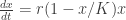
This is called the “logistic equation”.
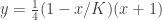
If you know some calculus you can solve the logistic equation by hand by separating the variables and integrating both sides; it’s a textbook exercise. The solutions are called “logistic functions”, and they look sort of like this:

The above graph shows the simplest solution:

of the simplest logistic equation in the world:

Here the carrying capacity is 1. Populations less than 1 sound a bit silly, so think of it as 1 million rabbits. You can see how the solution starts out growing almost exponentially and then levels off. There’s a very different-looking solution where the population starts off above the carrying capacity and decreases. There’s also a silly solution involving negative populations. But whenever the population starts out positive, it approaches the carrying capacity.
The solution where the population just stays at the carrying capacity:

is called a “stable equilibrium”, because it’s constant in time and nearby solutions approach it.
But now let’s introduce another species: some wolves, which eat the rabbits! So, let 

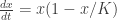
And before the wolves meet the rabbits, let’s assume they obey this equation:

so that their numbers would decay exponentially to zero if there were nothing to eat.
So far, not very interesting. But now let’s include a term that describes how predators eat prey. Let’s say that on top of the above effect, the predators grow in numbers, and the prey decrease, at a rate proportional to:

For small numbers of prey and predators, this means that predation increases nearly linearly with both
Okay, so let’s try these equations:

and
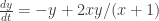
The constants 4 and 2 here have been chosen for simplicity rather than realism.
Before we plunge ahead and get a computer to solve these equations, let’s see what we can do by hand. Setting 
together with the boring line 
Setting 

together with the boring line 
The interesting parabola and the interesting line separate the 
which of course is an equilibrium, since 

So, if
We could figure this out analytically, but let’s look at two of Graham’s plots. Here’s a solution when 

The gray curves are the separatrices. The red curve shows a solution of the equations, with the numbers showing the passage of time. So, you can see that the solution spirals in towards the equilibrium. That’s what you expect of a stable equilibrium.
Here’s a picture when 

The red and blue curves are two solutions, again numbered to show how time passes. The red curve spirals in towards the dotted gray curve. The blue one spirals out towards it. The gray curve is also a solution. It’s called a “stable limit cycle” because it’s periodic, and nearby solutions move closer and closer to it.
With a bit more work, we could show analytically that whenever 
Now, what if we add noise? We saw the answer last week: where we before had a stable equilibrium, we now can get irregular cycles — because the noise keeps pushing the solution away from the equilibrium!
Here’s how it looks for 

The following graph shows a longer run in the noisy

There is irregular periodicity — and as you’d expect, the predators tends to lag behind the prey. A burst in the rabbit population causes a rise in the wolf population; a lot of wolves eat a lot of rabbits; a crash in rabbits causes a crash in wolves.
This sort of phenomenon is actually seen in nature sometimes. The most famous case involves the snowshoe hare and the lynx in Canada. It was first noted by MacLulich:
• D. A. MacLulich, Fluctuations in the Numbers of the Varying Hare (Lepus americanus), University of Toronto Studies Biological Series 43, University of Toronto Press, Toronto, 1937.
The snowshoe hare is also known as the “varying hare”, because its coat varies in color quite dramatically. In the summer it looks like this:

In the winter it looks like this:

The Canada lynx is an impressive creature:

But don’t be too scared: it only weighs 8-11 kilograms, nothing like a tiger or lion.
Down in the United States, the same species lynx went extinct in Colorado around 1973 — but now it’s back!
• Colorado Division of Wildlife, Success of the Lynx Reintroduction Program, 27 September, 2010.
In Canada, at least, the lynx rely for the snowshoe hare for 60% to 97% of their diet. I suppose this is one reason the hare has evolved such magnificent protective coloration. This is also why the hare and lynx populations are tightly coupled. They rise and crash in irregular cycles that look a bit like what we saw in our simplified model:
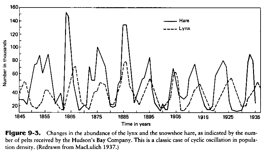
This cycle looks a bit more strongly periodic than Graham’s graph, so to fit this data, we might want to choose parameters that give a limit cycle rather than a stable equilibrium.
But I should warn you, in case it’s not obvious: everything about population biology is infinitely more complicated than the models I’ve showed you so far! Some obvious complications: snowshoe hare breed in the spring, their diet varies dramatically over the course of year, and the lynx also eat rodents and birds, carrion when it’s available, and sometimes even deer. Some less obvious ones: the hare will eat dead mice and even dead hare when they’re available, and the lynx can control the size of their litter depending on the abundance of food. And I’m sure all these facts are just the tip of the iceberg. So, it’s best to think of models here as crude caricatures designed to illustrate a few features of a very complex system.
I hope someday to say a bit more and go a bit deeper. Do any of you know good books or papers to read, or fascinating tidbits of information? Graham Jones recommends this book for some mathematical aspects of ecology:
• Michael R. Rose, Quantitative Ecological Theory, Johns Hopkins University Press, Maryland, 1987.
Alas, I haven’t read it yet.
Also: you can get Graham’s R code for predator-prey simulations at the Azimuth Project.
Under carefully controlled experimental circumstances, the organism will behave as it damned well pleases. – the Harvard Law of Animal Behavior


Nice post! I was wondering if can the hares adjust the time they change their fur, depending on the snowfall of that year? If not, irregular starts/endings of snowfall benefits the number of lynxes, though only in the short term…
I wanted to find some more details on how the hares change the color of their fur, but I didn’t have time — I’m going to Angkor Wat tomorrow, so I have to pack!
There could be some interesting regulation of gene expression going on here.
And yes, hares that didn’t change color at the right times would be a lot easier to catch, which would benefit the lynx. (I think the plural of ‘lynx’ is ‘lynx’.)
Of course this would put a huge evolutionary pressure on the hares to get good at changing color, once some of them could do it.
Meanwhile I googled a bit and found here:
> This color change, stimulated by the change in day length, takes about 10 weeks in the fall and spring.
So I guess they’re in bad luck if snowfall would come very irregularly (I was thinking if this could be one of the stochastic effects, in addition to food resources, but I thought snowfall would be more easily quantifiable).
Btw, Merriam-Webster has both lynx and lynxes.
Methinks you got rabbits and wolves mixed up when you first assigned them to x and y.
You may have read this post before I fixed some mistakes. Or maybe there are still some remaining mistakes? I want rabbits to be , wolves to be
  .
.
The sentence with wolves and rabbits around the wrong way in this one: “So, let x be the number of wolves, and y the number of rabbits.”
D’oh!
Thanks – fixed.
Although population dynamics as coupled differential equations can behave somewhat like “this sort of phenomenon is actually seen in nature”, it is important to keep in mind that populations are discrete and reproduce discretely. As you mention, even hares don’t reproduce continously. The typical search for better parameters of the wrong model usually should be directed instead to a better parameterization.
That being said, if the discretized version of the logistic equation is reformed into a logistic map
http://en.wikipedia.org/wiki/Logistic_map
it has too boring (constant) behavior. On the other hand, the continuumized version of the logistic map yields a logistic equation with too exciting (singular) behavior.
As Feigenbaum et al. investigated thoroughly, the discrete logistic map can exhibit chaos all by itself, i.e. just hares with no wolves. That is one example illustrating the general fact that nonlinear discrete equations have more complex behavior than nonlinear differential equations of the same order -essentially the discrete case parameters have to be very finely tuned to act like the differential case.
John F. wrote:
Yes! And that’s just one of many things we need to keep in mind. Here’s another. Rabbits and wolves are agents moving around in space in a complicated way; there’s not a constant ‘density of rabbits’ throughout the relevant ecosystem, so describing the rabbit population by a single number at each time is oversimplified.
My attitude is that we need a huge repertoire of models, all ‘oversimplified’ in one way or another, to begin to understand biological and ecological phenomena. The models provide insight into which mechanisms can give rise to which effects. If a model doesn’t give rise to some effects we see, we know it’s missing something. But if it does give rise to an effect we see, we can’t conclude it’s “right”.
This attitude has actually allowed me to relax and learn to enjoy simplified models for what they are, without hoping or expecting that they match reality very well.
Mathematicians should be allowed to study simple models without feeling guilty about the fact that these models are never “right”. Models are mathematical entities and worthy of study as such.
But scientists who care about what the models are modelling should try to always be aware of their models’ deficiencies, constantly on the lookout for data that their models don’t explain, constantly eager to test their models’ predictive power by means of statistical tests, and constantly eager to improve those models.
In This Week’s Finds I want to start by talking about lots of very simple models, because it’s these that everyone should understand: more complicated models are inevitably more specialized.
Yes, I’d love to talk about that someday! For now people can try the reference you mentioned:
• Logistic map, Wikipedia.
And indeed, late last night I read that someplace where lynxes went extinct, the hare population continued to exhibit dramatic cycles! I’ll try to find this again and add it to “week309”, because it’s a great example of how one can be fooled by the seeming “success” of a model into thinking one understands more than one really does!
John once again nails the issue. If you think about it, these same non-linear equations are operative in chemical reactions and they work extremely well in describing the dynamics. The difference of course is that the mixing of the reagents in solution is very thorough and entropy will drive this to uniformity rapidly. Nothing really like that occurs in ecosystems unless they happen to be very localized or located in a petri dish. No wonder that one of the famous studies of an eco-cycle occurred on tiny St. Matthew Island concerning a reindeer population.
So I think dispersion is very important on a larger scale.
The other odd part is that the Logistic sigmoid function is used also to model oil depletion and is recognized as the peak shape of Peak Oil. Yet if you look at what Graham Jones has described well with the logistic function is an asymptotic transition to a steady-state carrying capacity. But what does oil depletion decline to? Not a steady-state carrying capacity that’s for sure — it declines to zero!
So the traditionalists in the peak oil analysis community have changed the logistic definition to describe a cumulative oil production, not a current production level. This is equivalent to making the Logistic equation for biological entities follow a cumulative population level, which makes no sense as it would predict extinction for a species every time!
The math behind why this “trick” may kind-of work for oil is because the root growth function is an exponential then the cumulative of an exponential will remain an exponential. By fortuitous chance, this ends up working only for growth functions of the exponential form.
Why do I bring this up? Because the equivalent logistic function can also be generated by dispersion of exponential growth rates bounded by a distribution of dispersed asymptotic limits. This works great for analysis and it allows a variety of growth rates (not just an exponential). I have been working this problem the past few years and it seems to explain the nagging inexplicable details that drive people crazy with these equations.
So my point echoes what John says, in that we need these simple models, but what is perhaps most surprising is that these models can get even simpler. All we need to consider is the role of disorder and entropy in describing the environment. Just like there isn’t one rate governing a rabbit’s reproductive rate, there are many rates describing oil production. All these go into the mix and we end up describing these systems not always as non-linear chaotically driven, but as simple disordered systems governed by straightforward dispersive variants of growth.
Of course this will bring up the chaos versus disorder debate once again :) And then how it impacts climate science research of course :) :)
‘Oversimplified’ models are incredibly useful in human endeavour. These simplified models are much more useful than correct ones for the same reason that a 1:50000 map (which necessarily omits a lot of detail) is much more useful than a 1:1 map. For example, an economic model which takes 20 years to perfectly forecast the state of the economy 10 years from now is much less useful than one which takes one day to make an approximate (i.e. wrong) forecast.
Spatial heterogeneity has been studied widely in the context of population dynamics, e.g.
Click to access jtb_95.pdf
So much so, spatially explicit models tend to be student homework problems, kind of like Ising models in other contexts.
Again, simulations obviously tend to be of discrete models, even if some of them are discretized versions of continuum equations. And discrete models behave differently from continuum models, I claim especially in the presence of noise terms.
Just found some fascinating stochastics papers that might address the criticism above. It’s about a discrete, spatial variant of the Lotka-Volterra model. The basic model is very simple – but ultimately leads to quite sophisticated mathematical machinery (measure space valued martingales, super-Brownian motion, etc.).
• C. Neuhauser and S. Pacala An explicitly spatial version of the Lotka–Volterra model with interspecific competition. Ann. Appl. Probability 9 (1999), 1226–1259.
From abstract:
From the introduction:
One might criticize the simplicity – but it seems robust large scale qualitative results emerge independent of inexactness of modelling (physicists know that epistemic miracle). For there is sort of a central limit theorem:
• Ted Cox and Ed Perkins, Rescaled Lotka-Volterra models converge to super-Brownian motion, Annals of Probability 33 (2005), 904-947.
• Ted Cox and Edwin Perkins, Renormalization of the two-dimensional Lotka-Volterra Model, Ann. Appl. Probability 18 (2008), 747-812.
From a talk announcement by Ed Perkins:
Just found a monograph that survived the sale and giveaway of my math library long ago: T.M. Liggett, Interactive Particle Systems.
The system that started this business is the stochastic Ising model (Glauber 1963, Dobrushin 1971). And now there is Neuhauser & Pacala 1999.
So, here is a close connection between statistical mechanics and quantitative ecology!
Heck, I just googled “quantitative ecology”+”statistical mechanics” and found this paper (JB wanted to read another of Dewar’s papers…)
R.C. Dewar, A. Port, Statistical mechanics unifies different ecological patterns, J. Theor. Biol. 251 (2008), 389-403
Abstract:
Thanks for the references, Florifulgurator! I’m just back from Angkor Wat and it’ll take me a while to read these, but while there I made a lot of progress connecting quantum field theory to models like the Lotka-Volterra equation, so some of the papers you mention sound very intriguing.
And by the way, I think this one:
• C. Neuhauser and S. Pacala An explicitly spatial version of the Lotka–Volterra model with interspecific competition, Ann. Appl. Probability 9 (1999), 1226–1259.
is by the same Stephen Pacala who helped write that paper on stabiliation wedges — the one I’ve been repeatedly blogging about, here!
(And someone complained in one of the comments that Pacala and Socolow couldn’t do math.)
What’s super-Brownian motion? I’m having trouble finding out from the paper that mentions it. At first I thought it might be the supersymmetric analogue of Brownian motion, which is actually something I’ve spent a bunch of time pondering — it’s important in some proofs of the Atiyah-Singer index theorem. Now I think that’s not what it is: none of the usual buzzwords were showing up. So I’m clueless.
I hit the same problem and did some research.
Try this.
The key search term seems to be ‘Dawson-Watanabe’
Thanks, Roger! Perhaps because I’m in Singapore, or perhaps for some other reason, when I click on your link I get told I’ve “either reached a page that is unavailable for viewing, or reached my viewing limit” — so I can’t actually see anything there.
But okay: ‘Dawson-Watanabe’. Knowing the right buzzword can be invaluable! It’s dinnertime now, but sometime when I have more energy I may track down that lead.
On the other hand, I also wouldn’t mind if someone broke down and explained this stuff to me!
What’s so “super” about super-Brownian motion? If it’s not supersymmetric, could it be a supermartingale?
Let’s not forget superstatistics.
http://en.wikipedia.org/wiki/Superstatistics
It’s a continuous stochastic process with values in the space of finite Borel measures on (or perhaps a Riemannian manifold). Like Brownian motion it has the Laplacian as generator, in the sense of a martingale problem, where the Laplacian operates by turning a measure
into the functional
Thanks, Flori! But if it has the Laplacian as generator, just as Brownian motion does, how can it be anything other than Brownian motion?
It’s a different space (quite an infinite dimensional one – thus the silly “super”).
What I forgot to mention: Consider the measures with a smooth Radon-Nikodym density
  wrt. Lebesgue measure
  . On these the “measure Laplacian” acts in the usual way due to Green’s formula:
There is another, maybe less known way, to get instability into the model. Due to gestations periods, the reproduction rate of mammals can be thought of to also depend on some state in the past. Such delays cause the trajectory to oscillate around like drunk drivers (with their delayed reaction time).
The logistic map, mentioned by John Furey, is one very simple model with the behavior you mention. In that model, time proceeds in discrete steps, and the population change at each step depends on the population at that step. This could describe a situation where animals decide each spring how many kids to have. (It sounds silly, but they do adjust the size of their litters based on the food available.)
Another approach is a delay-differential equation, where time is continuous but the rate of population growth now depends on the conditions some time ago.
Both these models are discussed on the Azimuth Library, thanks in part to Miguel Carrión-Álvarez:
• Logistic equation, Azimuth Library.
Of course, many more complex models are possible!
In the vein of mentioning further factors outside the model, I gather one of the issues is that when prey levels are low the stress on predators is “more severe than just quadratic in the prey population”, since they’re expending more and more energy just to get their “share” of a more and more scarce food resource.
“First I’ll talk to the science fiction author and astrophysicist Gregory Benford. I’ll ask him about his ideas on ‘geoengineering’ — proposed ways of deliberately manipulating the Earth’s climate to counteract the effects of global warming”
We can’t even fix our economy, how are we going to “fix” global climate? How can people delude themselves into believing that they are so intelligent that they can “fix” something that they broke due to their lack of intelligence in the first place? Humans were ignorantly harming the environment all these many years until now, and all of a sudden they’ve become smart enough to fix it? That’s blatant nonsense. We do not understand weather enough to be able to accurately predict the weather three days from now, and we are going to fix the alleged global warming problem? The current Ice Age started up four-million years ago for reasons unknown, yet we know how and when it will end and we will even be the ones to end it?
Over a hundred years ago, CO2 levels were around 280ppm. They are now at 380ppm. That is a 50% increase, yet we have not seen a 50% increase in temperatures. CO2 is allegedly a very strong forcing (as opposed to feedback) component, yet a one degree change for a 50% increase does not sound very forceful at all. What about those other 280ppm? From the stories we hear about climate today, you would think all of the current greenhouse effect on the Earth (which amounts to a total of 60F) would be due to CO2, but you would be wrong. It only accounts for less than 10% or less than 6F of the greenhouse effect…so how is CO2 going to become the terrible and huge monster that is supposed to completely destroy the Earth a hundred years from now in a runaway greenhouse effect conflagration? Talk about science fiction…
At least you are going to be asking the right person this kind of question, since anthropomorphic global warming and geoengineering are based more on science fiction instead of science fact and seasoned experience. Nevertheless, It will be entertaining (in a Star Trek sorta way).
People ignorantly assume that the Earth is a museum and that nothing is ever supposed to change naturally. By their “reasoning”, we should all still be in the midst of the devastating and destructive Little Ice Age, the Age that ended in 1850, due to our vast and great influence in manipulating climate. If that were true, we should be thankful that we were able to successfully manipulate the climate, because without it, we wouldn’t be able to support the crops (and thereby populations) that we do today, and heating costs would be unaffordable in many areas (like England and the East Coast of USA).
And let’s not forget how people can lie with statistics. What does it mean that the “average” temperature of the Earth has risen a measly one-and-a-quarter degree in the last century? What it doesn’t mean is that this temperature rise has been uniformly spread everywhere. If you look at the actual data, the vast majority of this temperature rise has been over Greenland, with very little change anywhere else. And if you think about it, even if it were everywhere, a 1.26F degree change is insignificant — I live in Phoenix AZ and everyday I see a ten degree variation from one end of town to the other (and the differences in temperature do not occur in the same places). That difference has no detrimental effect whatsoever. I wonder how many people have ever noticed that ten degree difference before? How much of a temperature variation is there across your town? Try http://www.fullscreenweather.com and see what you’ve been missing. An actual 1.26 degree change in temperature is not significant to any of us. Only Greenland and a few choice mountain tops are affected, and not enough people live in those places to be affected by it, but that isn’t what the media is telling us. Obviously what the media is telling us isn’t believable.
NASA preached that the world was coming to a freezing end in the 70’s and then did an about-face in the 2000’s, claiming that they had more and better data than they had in the 70’s. So the Global Cooling crisis was proclaimed out of ignorance but how do they know if they have enough data yet? Do they have all the data there is to get? Maybe “more and better data” is still forthcoming and they will have to change their minds again? And just now all these people are now coming forth, and they all are more intelligent than NASA? NASA has no credibility when it comes to these kind of things, and they are the most intelligent organization on this planet, in regards to climatology.
We need to tell all these people that want to “fix” our climate, to mind their own business because you know what generally happens when someone who doesn’t know what they are doing tries to meddle in something they don’t understand? They only make it worse!
The world doesn’t need another stupid Hollywood “hero”.
Correction: Oops, I meant 30%, not 50%, for the CO2 increase, but even that isn’t a proper approximation in a math group…not that a typo would change my argument any but…okay, try 5/14ths or 35.7%.
Either way, a 35.7% increase in CO2 with only a 1.26F degree increase in temp is not world changing. It is so ho hum. Heck, if my wife raised the thermostat in my house by 1.26F, neither you nor I would notice.
It seems to be common to say “if temperature rose by 1 degree C (or some similar amount) no-one would notice”. Do you really mean that, or do you mean “it would not have a significant or deleterous effect”? I’m pretty sure that if the temperature in your house was increseased for a year there’d be noticeable effects, eg, you might find that you’d eaten less (due to the mildly increased temperature affecting your appetite), a change in how long the fruit in your fruit-bowl lasts before going moldy, you might notice you were wearing sweaters very marginally less, etc.
I’m not saying any of these effects would have any significant effect on your life, but it’s repeatedly boldly stated that no-one would notice a 1 degree rise in their home and I really can’t believe that would be true.
Since nobody ever notices a 1-degree temperature rise in their house, everyone here in Singapore can turn their thermostats up a degree and save a lot of money—with no bad effects whatsoever!
So, everyone should do it right now.
And then, since it’s a rule that nobody ever notices a mere 1-degree rise, everyone should do it again.
But seriously, sorites aside, I have the air conditioner in my room set at 27°C now because I’m being decadent and drinking a cup of hot coffee. I usually can take 28°C, but when drinking coffee that’s enough to make me sweaty, and I don’t like that. My wife and I sometimes have big arguments over whether to go for 27°C or 28°C. It makes a noticeable difference. Most people here go for something like 24°C or less, and think we’re crazy—but I’d rather save energy, do my bit for the environment, and be a bit less alienated from the outdoors, which typically hits 31°C in the day. The colder you keep it indoors, the hotter it seems outside!
Well, by that reasoning if a person doesn’t notice the effect it therefore has none, is similar to the belief that money does not cause any physical impacts because they are not directly visible to us.
You remember I posted and in discussion it was verified that the average BTU/$ globally is a direct measure of the average share of the energy uses that cause our environmental impacts. We don’t see it, but ~8000 btu’s of energy consumption would have significant irreversible environmental impacts. Because the costs of energy use (that we don’t measure) are clearly now growing much faster than the benefits, I expect they are greater in value than $1.
A Robinson wrote:
I agree that humans have a poor track record when it comes to predicting the effects of their interventions in the biosphere. However, I believe that if global warming becomes a problem that really hurts humanity, a lot of people will become desperate to try any fix that seems plausible. So, I think it’s important to start discussing geoengineering now. Regardless of where the discussion leads, it may be important. For example, if the conclusion is that we shouldn’t try geoengineering, maybe that means we should try something else (e.g., limiting carbon emissions).
As you note later, it’s about a 36% increase in CO2 levels. But nobody who studies this subject expects that to lead to a 36% increase in temperatures. The Earth’s temperature is obviously not even proportional to the amount of CO2 in the atmosphere: if it were, no CO2 at all would mean a temperature of absolute zero!
The relevant concept here is climate sensitivity. The climate sensitivity is the amount the average temperature rises when the the CO2 concentration doubles. The 4th IPCC report gives a figure of between 2 and 4.5 °C for the climate sensitivity.
In short, it’s a logarithmic thing. So, multiplying the CO2 level by 1.36 should increase the average temperature by about log2 1.36 ≃ .44 times the climate sensitivity. That’s between 0.88 and 2 °C.
This is just approximate, but it’s a lot better than expecting a temperature increase proportional to the increase in CO2 concentration.
Nobody sensible claims that global warming is going to ‘completely destroy the Earth’. Here’s some better information:
Click the links for more details.
Looking forward to geoengineering discussion. My favorite scheme is ocean spray vessels off dry coasts to greatly increase local evaporation rates. Nonstratospheric aerosols and humidity greatly affect local precipitation also, and dissolve out lots of atmospheric CO2 to boot.
Roy Soc had special issue “Geoscale Engineering”
http://rsta.royalsocietypublishing.org/content/366/188
2.toc
I think lately all ocean spray fountain schemes are deliberately misanalyzed to play up the Twomey effect and downplay evaporation.
John,
You probably meant to say that whenever 1 < K < 3 there is a stable equilibrium.
If anyone wants to try this in MATLAB or octave:
K=2.5;
dv=@(t,v) [v(1)*(1-v(1)/K)-4*v(1)*v(2)/(v(1)+1);-v(2)+2*v(1)*v(2)/(v(1)+1)];
[t,v]=ode45(dv,[0 50],[2 1]);
plot(v(:,1),v(:,2));axis([0 2.5 0 1.2])
Giampiero wrote:
Yes, I’ll fix that! Thanks!
Yes and it runs verbatim in sage’s R mode. Although Sage does uses an earlier version. See
http://www.sagenb.org/home/pub/2662
which has Graham Jones R code verbatim.
One thing that surprises me in this kind of model is that the focus in theoretical ecology on population characteristics, which seems half of the solution, but looking at the individual differences e.g. human beings reactions to global warming, seems to be better focus for other heterogeneous individual properties.
Why not bring up the difference between how behavioral systems and mathematical systems develop their reactions over time? Some of the reasons smart models of physical systems turn out to not be durable, for ending up missing important simple things, are themselves quite durable.
[…] a kind of catastrophe called a “Hopf bifurcation”. I explained all this in week308 and week309. There I was looking at some other equations, not the Lotka-Volterra equations. But their […]