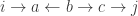
We’ve been looking at reaction networks, and we’re getting ready to find equilibrium solutions of the equations they give. To do this, we’ll need to connect them to another kind of network we’ve studied. A reaction network is something like this:

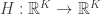
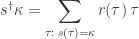
It’s a bunch of complexes, which are sums of basic building-blocks called species, together with arrows called transitions going between the complexes. If we know a number for each transition describing the rate at which it occurs, we get an equation called the ‘rate equation’. This describes how the amount of each species changes with time. We’ve been talking about this equation ever since the start of this series! Last time, we wrote it down in a new very compact form:

Here 


But now suppose we forget how each complex is made of species! Suppose we just think of them as abstract things in their own right, like numbered boxes:

We can use these boxes to describe states of some system. The arrows still describe transitions, but now we think of these as ways for the system to hop from one state to another. Say we know a number for each transition describing the probability per time at which it occurs:

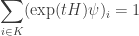
Then we get a ‘Markov process’—or in other words, a random walk where our system hops from one state to another. If 

This is simpler than the rate equation, because it’s linear. But the matrix
What’s the point? Well, our ultimate goal is to prove the deficiency zero theorem, which gives equilibrium solutions of the rate equation. That means finding

Today we’ll find all equilibria for the Markov process, meaning all

Then next time we’ll show some of these have the form

So, we’ll get

and thus
as desired!
So, let’s get to to work.
The Markov process of a graph with rates
We’ve been looking at stochastic reaction networks, which are things like this:

However, we can build a Markov process starting from just part of this information:

Let’s call this thing a ‘graph with rates’, for lack of a better name. We’ve been calling the things in 
Definition. A graph with rates consists of:
• a finite set of states

• a finite set of transitions

• a map 
• source and target maps 
Starting from this, we can get a Markov process describing how a probability distribution

for some Hamiltonian:
What is this Hamiltonian, exactly? Let’s think of it as a matrix where 


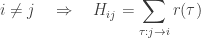
where we write 

Now, we saw in Part 11 that for a probability distribution to remain a probability distribution as it evolves in time according to the master equation, we need
The first condition holds already, and the second one tells us what the diagonal entries must be. So, we’re basically done describing 
Puzzle 1. Think of 

Equilibrium solutions of the master equation
Now we’ll classify equilibrium solutions of the master equation, meaning 
We’ll do only do this when our graph with rates is ‘weakly reversible’. This concept doesn’t actually depend on the rates, so let’s be general and say:
Definition. A graph is weakly reversible if for every edge 


This graph with rates is not weakly reversible:
but this one is:
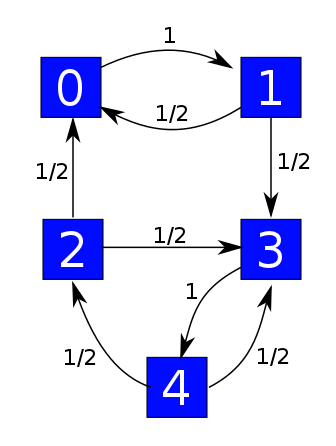
The good thing about the weakly reversible case is that we get one equilibrium solution of the master equation for each component of our graph, and all equilibrium solutions are linear combinations of these. This is not true in general! For example, this guy is not weakly reversible:

It has only one component, but the master equation has two linearly independent equilibrium solutions: one that vanishes except at the state 0, and one that vanishes except at the state 2.
The idea of a ‘component’ is supposed to be fairly intuitive—our graph falls apart into pieces called components—but we should make it precise. As explained in Part 21, the graphs we’re using here are directed multigraphs, meaning things like

where 

Two vertices
Remember, a directed path from

Here’s a path from 
and I hope you can write down the obvious but tedious definition of an ‘undirected path’, meaning a path made of edges that don’t necessarily point in the correct direction. Given that, we say two vertices 
For example,
Here’s a graph with one connected component and 3 strongly connected components, which are marked in blue:

For the theory we’re looking at now, we only care about connected components, not strongly connected components! However:
Puzzle 2. Show that for weakly reversible graph, the connected components are the same as the strongly connected components.
With these definitions out of way, we can state today’s big theorem:
Theorem. Suppose
Then for each connected component 


Moreover, these probability distributions 

Proof. We start by assuming our graph has one connected component. We use the Perron–Frobenius theorem, as explained in Part 20. This applies to ‘nonnegative’ matrices, meaning those whose entries are all nonnegative. That is not true of 

Since our graph is weakly reversible and has one connected component, it follows straight from the definitions that the operator
First, 


Subtracting 


We can show that in fact 

Since 
for all 

so we must have
We conclude that when our graph has one connected component, there is a probability distribution 


When 


This result must be absurdly familiar to people who study Markov processes, but I haven’t bothered to look up a reference yet. Do you happen to know a good one? I’d like to see one that generalizes this theorem to graphs that aren’t weakly reversible. I think I see how it goes. We don’t need that generalization right now, but it would be good to have around.
The Hamiltonian, revisited
One last small piece of business: last time I showed you a very slick formula for the Hamiltonian
We start with any graph with rates:
We extend 


We define the boundary operator just as we did last time:

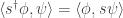
Then we put an inner product on the vector spaces 


where 


Then:
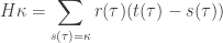
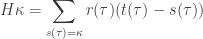
Theorem. The Hamiltonian for a graph with rates is given by

Proof. It suffices to check that this formula agrees with the formula for
Here we are using the complex 


First, we claim that
To prove this it’s enough to check that taking the inner products of either sides with any basis vector 
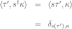
On the other hand:
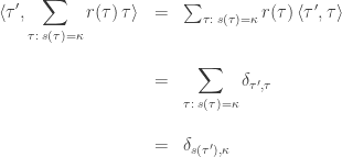
where the factor of 

Using this formula for 

which is precisely what we want. █
I hope you see through the formulas to their intuitive meaning. As usual, the formulas are just a way of precisely saying something that makes plenty of sense. If 


Okay, we’ve got all the machinery in place. Next time we’ll prove the deficiency zero theorem!


I think explanation has a typo since “the probability per time for our system to hop from the i state to the state j” doesn’t look backwards.
Yes, I guess my subconscious just couldn’t stomach the truth: is really the probability per time for our system to hop from the state
  to the state
Thanks—fixed!
For the puzzle: For any two vertices and
and  in a connected component of a weakly reversible graph we have an undirected path going from
  to
to  , a set of edges or transitions with sources and targets.
  . Starting with the edge attached to
  ,
,  , if
, if  then move to
  , if not then
  . Since the graph is weakly reversible there exists a directed path from
  to
to  , call this directed path
  (could be a composition of several transitions). Again move on to
  . Repeat until
  and then the set of primed and unprimed transitions
is a directed path from to
to  and since the graph is weakly reversible we have a directed path path back from
  to
to  for every pair of vertices in the connected component, hence it is strongly connected. What you really run into is exactly what you see in your example of an undirected path, namely vertices in the undirected path that are only the source or only the target for two different transitions, using weak reversibility on the one of these that goes with your ordering you end up with an ordered path. It’s interesting you can either choose to go along and use weak reversibility at each vertex to initially create a directed path back from
  to
to  or you can do what I did and use weak reversibility to direct your undirected path and then use weak reversibility again to show that component is strongly connected. Of course you need both for strongly connected.
sorry first time latex on here… and you missed a latex right at the end of the post.
Thanks for catching that—it’s those last-minute afterthoughts that get me, every time.
By the way, stuff like \usepackage, or macros don’t work here. You get what you get and that’s all you get. According to WordPress the blog comes pre-equipped with amsmath, amsfonts and amssymb. But they don’t list all the stuff that doesn’t work. All sorts of fancy formatting commands don’t work. So don’t push your luck.
If I understand your answer correctly, Blake, it sounds right. Let me say it my way.
We’ve got a connected component of a weakly reversible graph, and we’re trying to show it’s strongly connected. So, given two vertices v and w, we know there’s an undirected path of edges from v to w, and we’re trying to show there’s a directed one. Look at each edge in this path—say the edge between some vertex x and the next vertex on the path, y. Either it’s pointing the right way—from x to y—or it’s not. If it’s pointing the right way, don’t mess with it. If it’s pointing the wrong way—from y to x—we know by weak reversibility that there’s a directed path going back from x to y. So, replace this edge by that directed path.
We thus get a directed path from v to w, built from the edges in the original path that we pointing the right direction, and the directed paths we used to replace the edges that were pointing the wrong direction.
(Look, ma—no subscripts!)
By the way, maybe it’s time to announce that Blake Pollard is now starting grad school at U.C. Riverside! When are you actually going there, Blake?
I’m still working out here in Hawaii for about a month, staying island-side right up until the last minute! So I’ll be getting to Riverside probably the 21st of next month, just before classes start. Looking forward to it.
As for the puzzle I like your explanation better, I was trying to warm up my confusing math speak since its a bit rusty. The switching of certain edges with directed paths reminds me of time-ordering operators in QFT, except there you just switch the order of terms rather than replacing them with possibly more terms.
I’m showing up in Riverside on September 21st as well! See you in my ‘Math of Climate Science’ seminar.
Let me record here my guess about equilibria for general Markov processes on finite sets, where we drop the ‘weak reversibility’ assumption. Someone must know this already, and I’d love to see a reference.
A general directed multigraph looks a bit like this:
Actually this is just a directed graph: it doesn’t have multiple edges going from one vertex to another. It also doesn’t have edges from a vertex to itself. But as I’ve explained, these features are irrelevant for the Markov process! When studying Markov processes, it’s enough to consider directed graphs with positive numbers labelling their edges.
The strongly connected components are shaded in blue. If we collapse each strongly connected component to a point, and combine all edges from one component to another into a single edge, we get a directed acyclic graph, meaning a directed graph without any directed cycles.
What can the equilibria of the Markov process look like? In the terminology of this post, an equilibrium is a probability distribution with
with
A directed acyclic graph gives a partial order on the set of vertices, where v ≤ w exactly when there exists a directed path from v to w. Let’s say a vertex v is maximal if there’s no vertex w with v < w.
So, there's a partial order on the strongly connected components of a directed graph, and we can talk about a 'maximal' strongly connected component. In this picture:
the strongly connected component containing f and g is maximal.
If you imagine what happens with a probability distribution as it evolves in time according to a Markov process with the graph, you’ll see that probability will flow into this component, but never leave it.
In general there could be a bunch of maximal strongly connected components. Probability will flow into these, but never leave.
For this reason, I think it’s obvious that an equilibrium can only be nonzero on the strongly connected components that are maximal.
So what are these like? We can write the equilibrium as a sum of pieces, each supported on a different maximal strongly connected component. (By ‘supported on’ I mean that it’s zero outside this component.)
Each of these pieces will itself be an equilibrium—since no probability can flow out, and none will be flowing in from other maximal strongly connected components, either.
So, what’s an equilibrium like if it’s supported on just a single maximal strongly connected component?
Since each strongly connected component is connected and weakly reversible, the theorem I described in this post says there’s exactly one equilibrium probability distribution supported on this component. It’s positive everywhere, and every equilibrium
  is a scalar multiple of this.
Conclusion: for a general Markov process on a finite set, we get one equilibrium probability distribution supported on each maximal strongly connected component. Every equilibrium is a linear combination of these. They form a basis.