Milankovich vs the Ice Ages

guest post by Blake Pollard

Hi! My name is Blake S. Pollard. I am a physics graduate student working under Professor Baez at the University of California, Riverside. I studied Applied Physics as an undergraduate at Columbia University. As an undergraduate my research was more on the environmental side; working as a researcher at the Water Center, a part of the Earth Institute at Columbia University, I developed methods using time-series satellite data to keep track of irrigated agriculture over northwestern India for the past decade.

I am passionate about physics, but have the desire to apply my skills in more terrestrial settings. That is why I decided to come to UC Riverside and work with Professor Baez on some potentially more practical cross-disciplinary problems. Before starting work on my PhD I spent a year surfing in Hawaii, where I also worked in experimental particle physics at the University of Hawaii at Manoa. My current interests (besides passing my classes) lie in exploring potential applications of the analogy between information and entropy, as well as in understanding parallels between statistical, stochastic, and quantum mechanics.

Glacial cycles are one essential feature of Earth’s climate dynamics over timescales on the order of 100’s of kiloyears (kyr). It is often accepted as common knowledge that these glacial cycles are in some way forced by variations in the Earth’s orbit. In particular many have argued that the approximate 100 kyr period of glacial cycles corresponds to variations in the Earth’s eccentricity. As we saw in Professor Baez’s earlier posts, while the variation of eccentricity does affect the total insolation arriving to Earth, this variation is small. Thus many have proposed the existence of a nonlinear mechanism by which such small variations become amplified enough to drive the glacial cycles. Others have proposed that eccentricity is not primarily responsible for the 100 kyr period of the glacial cycles.

Here is a brief summary of some time series analysis I performed in order to better understand the relationship between the Earth’s Ice Ages and the Milankovich cycles.

I used publicly available data on the Earth’s orbital parameters computed by André Berger (see below for all references). This data includes an estimate of the insolation derived from these parameters, which is plotted below against the Earth’s temperature, as estimated using deuterium concentrations in an ice core from a site in the Antarctic called EPICA Dome C:

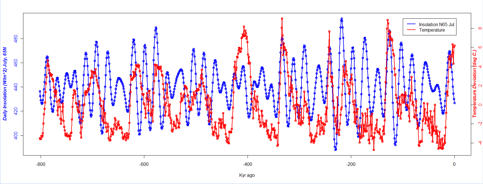
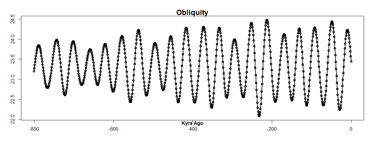
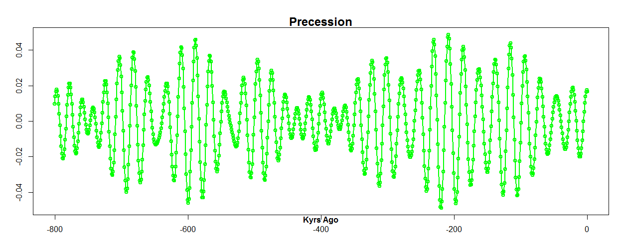
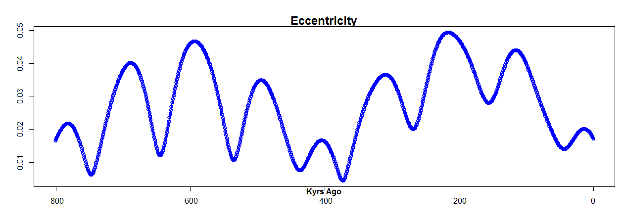
As you can see, it’s a complicated mess, even when you click to enlarge it! However, I’m going to focus on the orbital parameters themselves, which behave more simply. Below you can see graphs of three important parameters:

• obliquity (tilt of the Earth’s axis),
• precession (direction the tilted axis is pointing),
• eccentricity (how much the Earth’s orbit deviates from being circular).

You can click on any of the graphs here to enlarge them:

Richard Muller and Gordon MacDonald have argued that another astronomical parameter is important: the angle between the plane Earth’s orbit and the ‘invariant plane’ of the solar system. This invariant plane of the solar system depends on the angular momenta of the planets, but roughly coincides with the plane of Jupiter’s orbit, from what I understand. Here is a plot of the orbital plane inclination for the past 800 kyr:

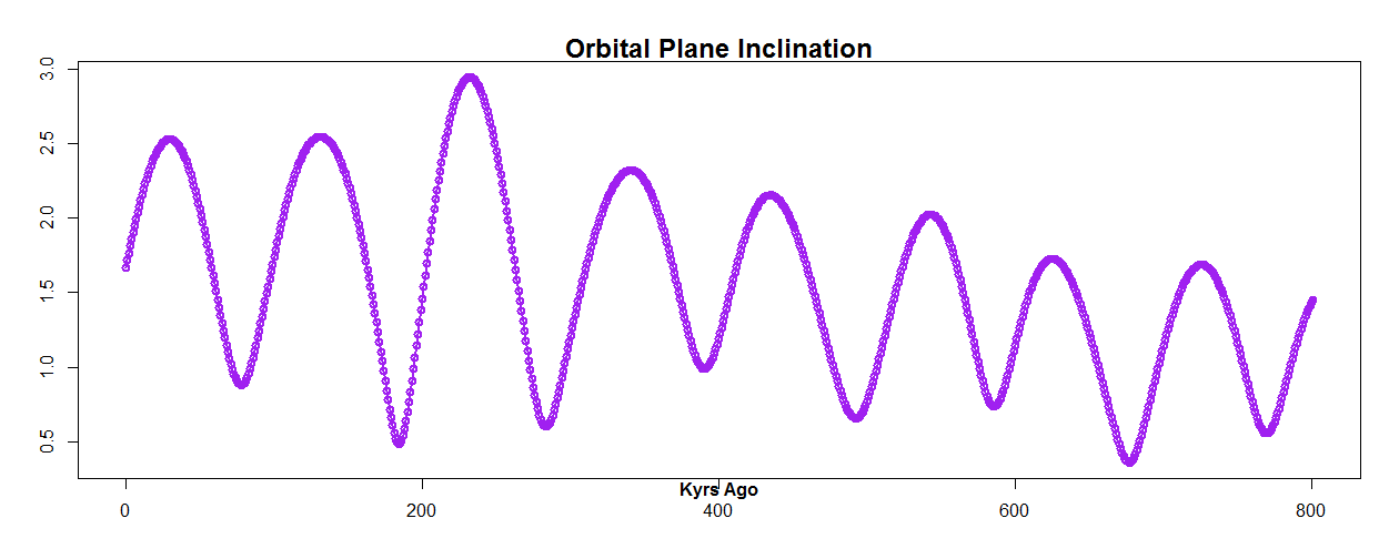
One can see from these plots, or from some spectral analysis, that the main periodicities of the orbital parameters are:

• Obliquity ~ 42 kyr
• Precession ~ 21 kyr
• Eccentricity ~100 kyr
• Orbital plane ~ 100 kyr

Of course the curves clearly are not simple sine waves with those frequencies. Fourier transforms give information regarding the relative power of different frequencies occurring in a time series, but there is no information left regarding the time dependence of these frequencies as the time dependence is integrated out in the Fourier transform.

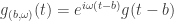
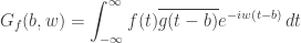
The Gabor transform is a generalization of the Fourier transform, sometimes referred to as the ‘windowed’ Fourier transform. For the Fourier transform:

one may think of , the ‘kernel function’, as the guy acting as your basis element in both spaces. For the Gabor transform instead of one defines a family of functions,

where is called the window function. Typical windows are square windows and triangular (Bartlett) windows, but the most common is the Gaussian:

which is used in the analysis below. The Gabor transform of a function is then given by

Note the output of a Gabor transform, like the Fourier transform, is a complex function. The modulus of this function indicates the strength of a particular frequency in the signal, while the phase carries information about the… well, phase.

For example the modulus of the Gabor transform of

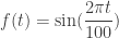
is shown below. For these I used the package Rwave, originally written in S by Rene Carmona and Bruno Torresani; R port by Brandon Whitcher.

You can see that the line centered at a frequency of .01 corresponds to the function’s period of 100 time units.

A Fourier transform would do okay for such a function, but consider now a sine wave whose frequency increases linearly. As you can see below, the Gabor transform of such a function shows the linear increase of frequency with time:

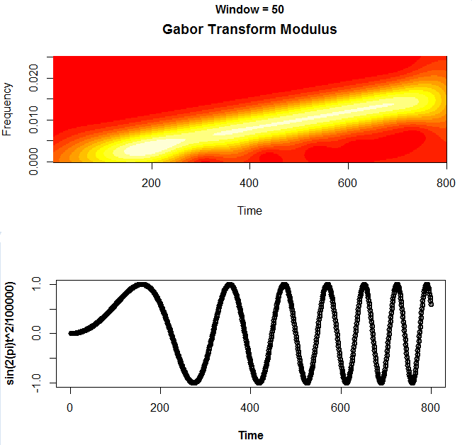
The window parameter in both of the above Gabor transforms is 100 time units. Adjusting this parameter effects the vertical blurriness of the Gabor transform. For example here is the same plot as a above, but with window parameters of 300, 200, 100, and 50 time units:

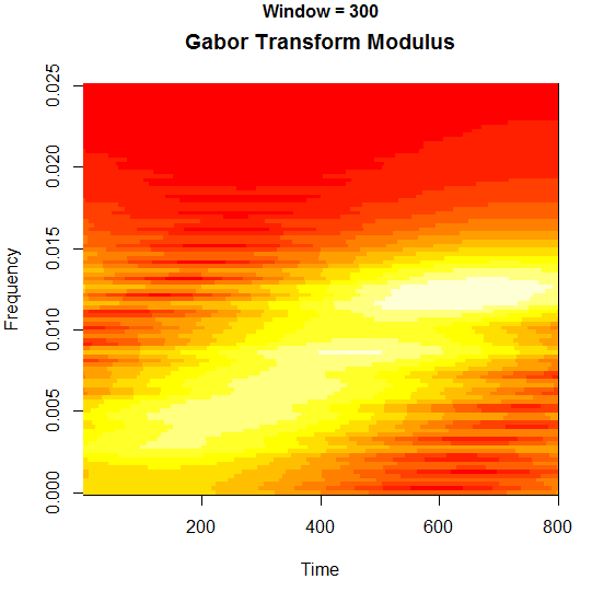
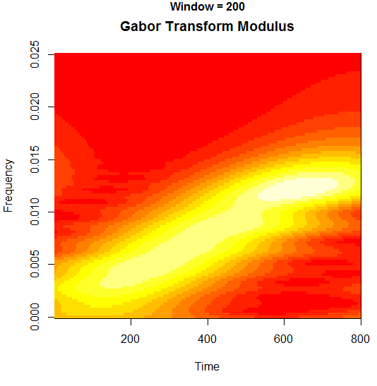
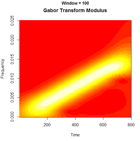
You can see as you make the window smaller the line gets sharper, but only to a point. When the window becomes approximately smaller than a given period of the signal the line starts to blur again. This makes sense, because you can’t know the frequency of a signal precisely at a precise moment in time… just like you can’t precisely know both the momentum and position of a particle in quantum mechanics! The math is related, in fact.

Now let’s look at the Earth’s temperature over the past 800 kyr, estimated from the EPICA ice core deuterium concentrations:

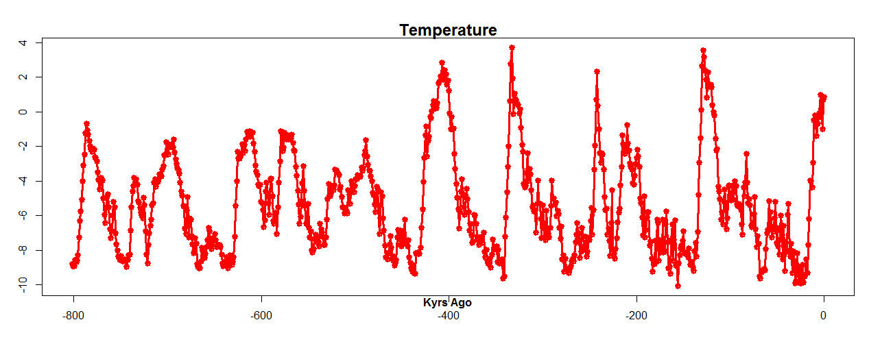
When you look at this, first you notice spikes occurring about every 100 kyr. You can also see that the last 5 of these spikes appear to be bigger and more dramatic than the ones occurring before 500 kyr ago. Roughly speaking, each of these spikes corresponds to rapid warming of the Earth, after which occurs slightly less rapid cooling, and then a slow decrease in temperature until the next spike occurs. These are the Earth’s glacial cycles.

At the bottom of the curve, where the temperature is about about 4 °C cooler than the mean of this curve, glaciers are forming and extending down across the northern hemisphere. The relatively warm periods on the top of the spikes, about 10 °C hotter than the glacial periods. are called the interglacials. You can see that we are currently in the middle of an interglacial, so the Earth is relatively warm compared to rest of the glacial cycles.

Now we’ll take a look at the windowed Fourier transform, or the Gabor transform, of this data. The window size for these plots is 300 kyr.

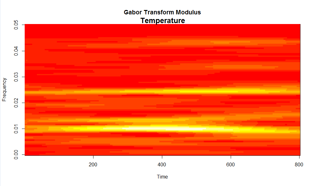
Zooming in a bit, one can see a few interesting features in this plot:

We see one line at a frequency of about .024, with a sampling rate of 1 kyr, corresponds to a period of about 42 kyr, close to the period of obliquity. We also see a few things going on around a frequency of .01, corresponding to a 100 kyr period.

The band at .024 appears to be relatively horizontal, indicating an approximately constant frequency. Around the 100 kyr periods there is more going on. At a slightly higher frequency, about .015, there appears to be a band of slowly increasing frequency. Also, around .01 it’s hard to say what is really going on. It is possible that we see a combination of two frequency elements, one increasing, one decreasing, but almost symmetric. This may just be an artifact of the Gabor transform or the window and frequency parameters.

The window size for the plots below is slightly smaller, about 250 kyr. If we put the temperature and obliquity Gabor Transforms side by side, we see this:

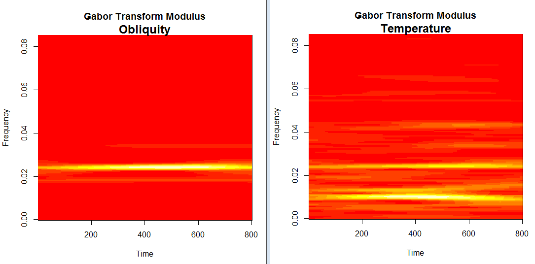
It’s clear the lines at .024 line up pretty well.

Doing the same with eccentricity:

Eccentricity does not line up well with temperature in this exercise though both have bright bands above and below .01 .

Now for temperature and orbital inclination:

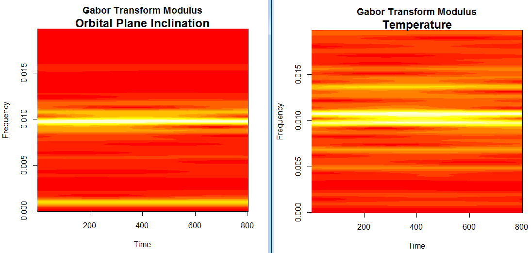
One sees that the frequencies line up better for this than for eccentricity, but one has to keep in mind that there is a nonlinear transformation performed on the ‘raw’ orbital plane data to project this down into the ‘invariant plane’ of the solar system. While this is physically motivated, it surely nudges the spectrum.

The temperature data clearly has a component with a period of approximately 42 kyr, matching well with obliquity. If you tilt your head a bit you can also see an indication of a fainter response at a frequency a bit above .04, corresponding roughly to period just below 25 kyrs, close to that of precession.

As far as the 100 kyr period goes, which is the periodicity of the glacial cycles, this analysis confirms much of what is known, namely that we can’t say for sure. Eccentricity seems to line up well with a periodicity of approximately 100 kyr, but on closer inspection there seems to be some discrepancies if you try to understand the glacial cycles as being forced by variations in eccentricity. The orbital plane inclination has a more similar Gabor transform modulus than does eccentricity.

A good next step would be to look the relative phases of the orbital parameters versus the temperature, but that’s all for now.

If you have any questions or comments or suggestions, please let me know!

References

The orbital data used above is due to André Berger et al and can be obtained here:

• Orbital variations and insolation database, NOAA/NCDC/WDC Paleoclimatology.

The temperature proxy is due to J. Jouzel et al, and it’s based on changes in deuterium concentrations from the EPICA Antarctic ice core dating back over 800 kyr. This data can be found here:

• EPICA Dome C – 800 kyr deuterium data and temperature estimates, NOAA Paleoclimatology.

Here are the papers by Muller and Macdonald that I mentioned:

• Richard Muller and Gordan MacDonald, Glacial cycles and astronomical forcing, Science 277 (1997), 215–218.

• Richard Muller and Gordan MacDonald, Spectrum of 100-kyr glacial cycle: orbital inclination, not eccentricity, PNAS 1997, 8329–8334.

They also have a book:

• Richard Muller and Gordan MacDonald, Ice Ages and Astronomical Causes, Springer, Berlin, 2002.

You can also get files of the data I used here:

• Berger et al orbital parameter data, with explanatory text here.

• Jouzel et al EPICA Dome C temperature data, with explanatory text here.

• Muller and Macdonald’s orbital plane inclination data.