
Today I’d like to wrap up my discussion of how to implement the Game of Life in our agent-based model software called AlgebraicABMs.
Kris Brown’s software for the Game of Life is here:
• game_of_life: code and explanation of the code.
He now has carefully documented the code to help you walk through it, and to see it in a beautiful format I recommend clicking on ‘explanation of the code’.
A fair amount of the rather short program is devoted to building the grid on which the Game of Life runs, and displaying the game as it runs. Instead of talking about this in detail—for that, read Kris Brown’s documentation!—I’ll just explain some of the underlying math.
In Part 10, I explained ‘C-sets’, which we use to represent ‘combinatorial’ information about the state of the world in our agent-based models. By ‘combinatorial’ I mean things that can be described using finite sets and maps between finite sets, like:
• what is the set of people in the model?
• for each person, who is their father and mother?
• for each pair of people, are they friends?
• what are the social networks by which people interact?
and so on.
But in addition to combinatorial information, our models need to include quantitative information about the state of the world. For example, entities can have real-valued attributes, integer-valued attributes and so on:
• people have ages and incomes,
• reservoirs have water levels,
and so on. To represent all of these we use ‘attributed C-sets’.
Attributed C-sets are an important data structure available in AlgebraicJulia. They have already been used to handle various kinds of networks that crucially involve quantitative information, e.g.
• Petri nets where each species has a ‘value’ and each transition has a `rate constant’
• ‘stock-flow diagrams where each stock has a ‘value’ and each flow has a `flow function’.
In the Game of Life we are using attributed C-sets in a milder way. Our approach to the Game of Life lets the cells be vertices of an arbitrary graph. But suppose we want that graph to be a square grid, like this:

Yes, this is a bit unorthodox: the cells are shown as circles rather than squares, and we’re drawing edges between them to say which are neighbors of which. Green cells are live; red cells are dead.
But my point here is that to display this picture, we want the cells to have x and y coordinates! And we can treat these coordinates as ‘attributes’ of the cells.
We’re using attributes in a ‘mild’ way here because the cells’ coordinates don’t change with time—and they don’t even show up in the rules for the Game of Life, so they don’t affect how the state of the world changes with time. We’re only using them to create a picture of the state of the world. But in most agent-based models, attributes will play a more significant role. So it’s good to talk about attributes.
Here’s how we get cells to have coordinates in AlgebraicJulia. First we do this:
@present SchLifeCoords <: SchLifeGraph begin
  Coords::AttrType
  coords::Attr(V, Coords)
end
Here we are taking the schema SchLifeGraph, which I explained in Part 10 and which looks like this:
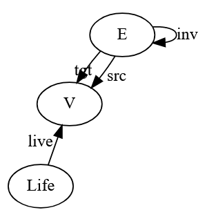
and we’re making this schema larger by giving the object V (for ‘vertex’) an attribute called coords:
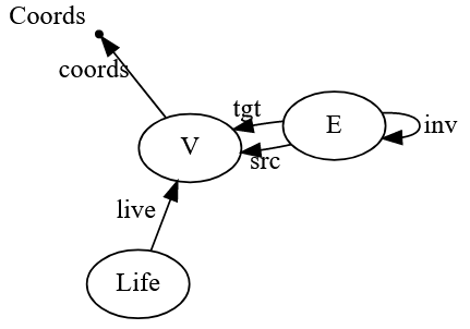
Note that Coords looks like just another object in our schema, and it looks like our schema has another morphism
However, Coords is not just any old object in our schema: it’s an ‘attribute type’. And coords: V → Coords is not just any old morphism: it’s an ‘attribute’. And now I need to tell you what these things mean!
Simply put, while an instance of our schema will assign arbitrary finite sets to V and E (since a graph can have an arbitrary finite set of vertices and edges), Coords will be forced to be a particular set, which happens not to be finite, namely the set of pairs of integers, ℤ2.
In the code, this happens here:
@acset_type LifeStateCoords(SchLifeCoords){Tuple{Int,Int}} <:
           AbstractSymmetricGraph;
You can see that the type ‘pair of integers’ is getting invoked. There’s also some more mysterious stuff going on. But instead of explaining that stuff, let me say more about the math of attributed C-sets. What are they, really?
Attributed C-sets
Attributed C-sets were introduced here:
• Evan Patterson, Owen Lynch and James Fairbanks, Categorical data structures for technical computing, Compositionality 4 5 (2022).
and further explained here:
• Owen Lynch, The categorical scoop on attributed C-sets, AlgebraicJulia blog, 5 October 2020.
The first paper gives two ways of thinking about attributed C-sets, and Owen’s paper gives a third more sophisticated way. I will go in the other direction and give a less sophisticated way.
I defined schemas and their instances in Part 10; now let me generalize all that stuff.
Remember, I said that a schema consists of:
1) a finite set of objects,
2) a finite set of morphisms, where each morphism goes from some object to some other object: e.g. if x and y are objects in our schema, we can have a morphism f: x → y, and
3) a finite set of equations between formal composites of morphisms in our schema: e.g. if we have morphisms f: x → y, g: y → z and h: x → z in our schema, we can have an equation h = g ∘ f.
Now we will add on an extra layer of structure, namely:
4) a subset of objects called attribute types, and
5) a subset of morphisms f: x → y called attributes where y is an attribute type and x is not, and
6) a set K(x) for each attribute type.
Mathematically K(x) is often an infinite set, like the integers ℤ or real numbers ℝ. But in AlgebraicJulia, K(x) can be any data type that has elements, e.g. Int (for integers) or Float32 (for single-precision floating-point numbers).
People still call this more elaborate thing a schema, though as a mathematician that makes me nervous.
An instance of this more elaborate kind of schema consists of:
1) a finite set F(x) for each object in the schema, and
2) a function F(f): F(x) → F(y) for each morphism in the schema, such that
3) whenever composites of morphisms in the schema obey an equation, their corresponding functions obey the corresponding equation, e.g. if h = g ∘ f in the schema then F(h) = F(g) ∘ F(f), and
4) F(x) = K(x) when x is an attribute type.
If our schema presents some category C, we also call an instance of it an attributed C-set.
But I hope you understand the key point. This setup gives us a way to ‘nail down’ the set F(x) when x is an attribute type, forcing it to equal the same set K(x) for every instance F. In the Game of Life, we choose
This forces
for every instance F. This in turn forces the coordinates of every vertex v ∈ F(V) to be a pair of integers for every instance F—that is, for every state of the world in the Game of Life.
This is all I will say about our implementation of the Game of Life. It’s rather atypical as agent-based models go, so while it illustrates many aspects of our methodology, for others we’ll need to turn to some other models. Xiaoyan Li has been working hard on some models of pertussis (whooping cough), so I should talk about those.

