Agent-Based Models (Part 8)

Last time I presented a class of agent-based models where agents hop around a graph in a stochastic way. Each vertex of the graph is some ‘state’ agents can be in, and each edge is called a ‘transition’. In these models, the probability per time of an agent making a transition and leaving some state can depend on when it arrived at that state. It can also depend on which agents are in other states that are ‘linked’ to that edge—and when those agents arrived.

I’ve been trying to generalize this framework to handle processes where agents are born or die—or perhaps more generally, processes where some number of agents turn into some other number of agents. There’s already a framework that does something sort of like this. It’s called ‘stochastic Petri nets’, and we explained this framework here:

• John Baez and Jacob Biamonte, Quantum Techniques for Stochastic Mechanics, World Scientific Press, Singapore, 2018. (See also blog articles here.)

However, in their simplest form, stochastic Petri nets are designed for agents whose only distinguishing information is which state they’re in. They don’t have ‘names’—that is, individual identities. Thus, even calling them ‘agents’ is a bit of a stretch: usually they’re called ‘tokens’, since they’re drawn as black dots.

We could try to enhance the Petri net framework to give tokens names and other identifying features. There are various imaginable ways to do this, such as ‘colored Petri nets’. But so far this approach seems rather ill-adapted for processes where agents have identities—perhaps because I’m not thinking about the problem the right way.

So, at some point I decided to try something less ambitious. It turns out that in applications to epidemiology, general processes where n agents come in and m go out are not often required. So I’ve been trying to minimally enhance the framework from last time to include processes ‘birth’ and ‘death’ processes as well as transitions from state to state.

As I thought about this, some questions kept plaguing me:

When an agent gets created, or ‘born’, which one actually gets born? In other words, what is its name? Its precise name may not matter, but if we want to keep track of it after it’s born, we need to give it a name. And this name had better be ‘fresh’: not already the name of some other agent.

There’s also the question of what happens when an agent gets destroyed, or ‘dies’. This feels less difficult: there just stops being an agent with the given name. But probably we want to prevent a new agent from having the same name as that dead agent.

Both these questions seem fairly simple, but so far they’re making it hard for me to invent a truly elegant framework. At first I tried to separately describe transitions between states, births, and deaths. But this seemed to triplicate the amount of work I needed to do.

Then I tried models that have

• a finite set of states,

• a finite set of transitions,

• maps mapping each transition to its upstream and downstream states.

Here is the disjoint union of and a singleton whose one element is called undefined. Maps from to are a standard way to talk about partially defined maps from to We get four cases:

1) If the downstream of a transition is defined (i.e. in ) but its upstream is undefined we call this transition a birth transition.

2) If the upstream of a transition is defined but its downstream is undefined we call this transition a death transition.

3) If the upstream and downstream of a transition are both defined we call this transition a transformation. In practice most of transitions will be of this sort.

4) We never need transitions whose upstream and downstream are undefined: these would describe agents that pop into existence and instantly disappear.

This is sort of nice, except for the fourth case. Unfortunately when I go ahead and try to actually describe a model based on this paradigm, I seem still to wind up needing to handle births, deaths and transformations quite differently.

For example, last time my models had a fixed set of agents. To handle births and deaths, I wanted to make this set time-dependent. But I need to separately say how this works for transformations, birth transitions and death transitions. For transformations we don’t change For birth transitions we add a new element to And for death transitions we remove an element from and maybe record its name on a ledger or drive a stake through its heart to make sure it can never be born again!

So far this is tolerable, but things get worse. Our model also needs ‘links’ from states to transitions, to say how agents present in those states affect the timing of those transition. These are used in the ‘jump function’, a stochastic function that answers this question:

If at time agent arrives at the state upstream to some transition and the agents at states linked to the transition form some set when will agent make the transition given that it doesn’t do anything else first?

This works fine for transformations, meaning transitions that have both an upstream and downstream state. It works just a tiny bit differently for death transitions. But birth transitions are quite different: since newly born agents don’t have a previous upstream state , they don’t have a time at which they arrived at that state.

Perhaps this is just how modeling works: perhaps the search for a staggeringly beautiful framework is a distraction. But another approach just occurred to me. Today I just want to briefly state it. I don’t want to write a full blog article on it yet, since I’ve already spent a lot of time writing two articles that I deleted when I became disgusted with them—and I might become disgusted with this approach too!

Briefly, this approach is exactly the approach I described last time. There are fundamentally no births and no deaths: all transitions have an upstream and a downstream state. There is a fixed set of agents that does not change with time. We handle births and deaths using a dirty trick.

Namely, births are transitions out of a ‘unborn’ state. Agents hang around in this state until they are born.

Similarly, deaths are transitions to a ‘dead’ state.

There can be multiple ‘unborn’ states and ‘dead’ states. Having multiple unborn states makes it easy to have agents with different characteristics enter the model. Having multiple dead states makes it easy for us to keep tallies of different causes of death. We should make the unborn states distinct from the dead states to prevent ‘reincarnation’—that is, the birth of a new agent that happens to equal an agent that previously died.

I’m hoping that when we proceed this way, we can shoehorn birth and death processes into the framework described last time, without really needing to modify it at all! All we’re doing is exploiting it in a new way.

Here’s one possible problem: if we start with a finite number of agents in the ‘unborn’ states, the population of agents can’t grow indefinitely! But this doesn’t seem very dire. For most agent-based models we don’t feel a need to let the number of agents grow arbitrarily large. Or we can relax the requirement that the set of agents is finite, and put an infinite number of agents in an unborn state. This can be done without using an infinite amount of memory: it’s a ‘potential infinity’ rather than an ‘actual infinity’.

There could be other problems. So I’ll post this now before I think of them.

Protonium

It looks like they’ve found protonium in the decay of a heavy particle!

Protonium is made of a proton and an antiproton orbiting each other. It lasts a very short time before they annihilate each other.

It’s a bit like a hydrogen atom where the electron has been replaced with an antiproton! But it’s much smaller than a hydrogen atom. And unlike a hydrogen atom, which is held together by the electric force, protonium is mainly held together by the strong nuclear force.

There are various ways to make protonium. One is to make a bunch of antiprotons and mix them with protons. This was done accidentally in 2002. They only realized this upon carefully analyzing the data 4 years later.

This time, people were studying the decay of the J/psi particle. The J/psi is made of a heavy quark and its antiparticle. It’s 3.3 times as heavy as a proton, so it’s theoretically able to decay into protonium. And careful study showed that yes, it does this sometimes!

The new paper on this has a rather dry title—not “We found protonium!” But it has over 550 authors, which hints that it’s a big deal. I won’t list them.

• BESIII Collaboration, Observation of the anomalous shape of X(1840) in J/ψ→γ3(π+π−), Phys. Rev. Lett. 132 (2024), 151901.

The idea here is that sometimes the J/ψ particle decays into a gamma ray and 3 pion-antipion pairs. When they examined this decay, they found evidence that an intermediate step involved a particle of mass 1880 MeV/c², a bit more than an already known intermediate of mass 1840 MeV/c².

This new particle is a bit lighter than twice the mass of a proton, 938 MeV/c². So, there’s a good chance that it’s protonium!

But how did physicists made protonium by accident in 2002? They were trying to make antihydrogen, which is a positron orbiting an antiproton. To do this, they used the Antiproton Decelerator at CERN. This is just one of the many cool gadgets they keep near the Swiss-French border.

You see, to create antiprotons you need to smash particles at each other at almost the speed of light—so the antiprotons usually shoot out really fast. It takes serious cleverness to slow them down and catch them without letting them bump into matter and annihilate.

That’s what the Antiproton Decelerator does. So they created a bunch of antiprotons and slowed them down. Once they managed to do this, they caught the antiprotons in a Penning trap. This holds charged particles using magnetic and electric fields. Then they cooled the antiprotons—slowed them even more—by letting them interact with a cold gas of electrons. Then they mixed in some positrons. And they got antihydrogen!

But apparently some protons got in there too, so they also made some protonium, by accident. They only realized this when they carefully analyzed the data 4 years later, in a paper with only a few authors:

• N. Zurlo, M. Amoretti, C. Amsler, G. Bonomi, C. Carraro, C. L. Cesar, M. Charlton, M. Doser, A. Fontana, R. Funakoshi, P. Genova, R. S. Hayano, L. V. Jorgensen, A. Kellerbauer, V. Lagomarsino, R. Landua, E. Lodi Rizzini, M. Macri, N. Madsen, G. Manuzio, D. Mitchard, P. Montagna, L. G. Posada, H. Pruys, C. Regenfus, A. Rotondi, G. Testera, D. P. Van der Werf, A. Variola, L. Venturelli and Y. Yamazaki, Production of slow protonium in vacuum, Hyperfine Interactions 172 (2006), 97–105.

Protonium is sometimes called an ‘exotic atom’—though personally I’d consider it an exotic nucleus. The child in me thinks it’s really cool that there’s an abbreviation for protonium, Pn, just like a normal element.

T Corona Borealis

 

Sometime this year, the star T Corona Borealis will go nova and become much brighter! At least that’s what a lot of astronomers think. So examine the sky between Arcturus and Vega now—and look again if you hear this event has happened. Normally this star is magnitude 10, too dim to see. When it goes nova is should reach magnitude 2 for a week—as bright as the North Star. So you will see a new star, which is the original meaning of ‘nova’.

But why do they think T Corona Borealis will go nova this year? How could they possibly know that?

It’s done this before. It’s a binary star with a white dwarf orbiting a red giant. The red giant is spewing out gas. The much denser white dwarf collects some of this gas on its surface until there’s enough fuel to cause a runaway thermonuclear reaction—a nova!

We’ve seen it happen twice. T Corona Borealis went nova on May 12, 1866 and again on February 9, 1946. What’s happening now is a lot like what happened in 1946.

In February 2015, there was a sustained brightening of T Corona Borealis: it went from magnitude 10.5 to about 9.2. The same thing happened eight years before it went nova the last time.

In June 2018, the star dimmed slightly but still remained at an unusually high level of activity. Then in April 2023 it dimmed to magnitude 12.3. The same thing happened one year before it went nova the last time.

If this pattern continues, T Corona Borealis should erupt sometime between now and September 2024. I’m not completely confident that it will follow the same pattern! But we can just wait and see.

This is one of only 5 known repeating novas in the Milky Way, so we’re lucky to have this chance.

Here’s how it might work:

The description at NASA’s blog:

A red giant star and white dwarf orbit each other in this animation of a nova. The red giant is a large sphere in shades of red, orange, and white, with the side facing the white dwarf the lightest shades. The white dwarf is hidden in a bright glow of white and yellows, which represent an accretion disk around the star. A stream of material, shown as a diffuse cloud of red, flows from the red giant to the white dwarf. The animation opens with the red giant on the right side of the screen, co-orbiting the white dwarf. When the red giant moves behind the white dwarf, a nova explosion on the white dwarf ignites, filling the screen with white light. After the light fades, a ball of ejected nova material is shown in pale orange. A small white spot remains after the fog of material clears, indicating that the white dwarf has survived the explosion.

For more details, try this:

• B. E. Schaefer, B. Kloppenborg, E. O. Waagen and the AAVSO observers, Announcing T CrB pre-eruption dip, AAVSO News and Announcements.

The Probability of Undecidability

There’s a lot we don’t know. There’s a lot we can’t know. But can we at least know how much we can’t know?

What fraction of mathematical statements are undecidable—that is, can be neither proved nor disproved? There are many ways to make this question precise… but it remains a bit mysterious. The best results I know appear, not in a published paper, but on MathOverflow!

In 1998, the Fields-medal winning topologist Michael Freedman conjectured that the fraction of statements that are provable in Peano Arithmetic approaches zero quite rapidly as you go to longer and longer statements:

 

 

He must also have been conjecturing that Peano Arithmetic is consistent, since if it’s inconsistent then all its statements are provable. From now on let’s assume that PA is consistent.

In 2005, Cristian Calude and Konrad Jürgensen published a paper arguing that Freedman was on the right track. More precisely, they showed that the fraction of statements in PA that are provable goes to zero as we go to longer and longer statements. The fraction of disprovable statements also goes to zero. So, the fraction of undecidable statements approaches 1.

Unfortunately their paper had a mistake!

In 2009, David Speyer argued that the fraction of provable statements does not approach 0 and does not approach 1 as we consider longer and longer statements. Instead, it’s bounded by numbers between 0 and 1. Similarly for the fraction of undecidable statements! His argument is not air-tight, as he admits and explains—but I believe it. Someone should try to complete his proof.

Speyer’s idea is very simple: if P is any statement, the statement “P or 1 = 1” is provable. This can be used to get a lower bound on the number of provable statements of a given length. Similarly, suppose G is some undecidable statement. Then for any statement P, the statement “G and (P or 1 = 1)” is undecidable. This can be used to get a lower bound on the number of undecidable statements of a given length.

The Probability of the Law of Excluded Middle

The Law of Excluded Middle says that for any statement P, “P or not P” is true.

Is this law true? In classical logic it is. But in intuitionistic logic it’s not.

So, in intuitionistic logic we can ask what’s the probability that a randomly chosen statement obeys the Law of Excluded Middle. And the answer is “at most 2/3—or else your logic is classical”.

This is a very nice new result by Benjamin Bumpus and Zoltan Kocsis:

• Benjamin Bumpus, Degree of classicality, Merlin’s Notebook, 27 February 2024.

Of course they had to make this more precise before proving it. Just as classical logic is described by Boolean algebras, intuitionistic logic is described by something a bit more general: Heyting algebras. They proved that in a finite Heyting algebra, if more than 2/3 of the statements obey the Law of Excluded Middle, then it must be a Boolean algebra!

Interestingly, nothing like this is true for “not not P implies P”. They showed this can hold for an arbitrarily high fraction of statements in a Heyting algebra that is still not Boolean.

Here’s a piece of the free Heyting algebra on one generator, which some call the Rieger–Nishimura lattice:

Taking the principle of excluded middle from the mathematician would be the same, say, as proscribing the telescope to the astronomer or to the boxer the use of his fists. — David Hilbert

I disagree with this statement, but boy, Hilbert sure could write!

Nicholas Ludford

At first glance it’s amazing that one of the great British composers of the 1400s largely sank from view until his works were rediscovered in 1850.

But the reason is not hard to find. When the Puritans took over England, they burned not only witches and heretics, but also books — and music! They hated the complex polyphonic choral music of the Catholics.

So, in the history of British music, between the great polyphonists Robert Fayrfax (1465-1521) and John Taverner (1490-1545), there was a kind of gap — a silence — until the Peterhouse Partbooks were rediscovered.

These were an extensive collection of musical manuscripts, handwritten by a single scribe between 1539 and 1541. Most of them got lost somehow and found only in the 1850s. Others were found even later, in 1926! They were hidden behind a panel in a library — probably hidden from the Puritans.

The 1850 batch contains wonderful compositions by Nicholas Ludford
(~1485-1557). One music scholar has called him “one of the last unsung
geniuses of Tudor polyphony”. Another wrote:

it is more a matter of astonishment that such mastery should be displayed by a composer of whom virtually nothing was known until modern times.

Ludford’s work was first recorded only in 1993, and much of the Peterhouse Partbooks have been recorded only more recently. A Boston group called Blue Heron released a 5-CD set, starting in 2010 and ending in 2017. It’s magnificent!

Below you can hear the Sanctus from Nicholas Ludford’s Missa Regnum mundi. It has long, sleek lines of harmony; you can lose yourself trying to follow all the parts.

Agent-Based Models (Part 7)

Last time I presented a simple, limited class of agent-based models where each agent independently hops around a graph. I wrote:

Today the probability for an agent to hop from one vertex of the graph to another by going along some edge will be determined the moment the agent arrives at that vertex. It will depend only on the agent and the various edges leaving that vertex. Later I’ll want this probability to depend on other things too—like whether other agents are at some vertex or other. When we do that, we’ll need to keep updating this probability as the other agents move around.

Let me try to figure out that generalization now.

Last time I discovered something surprising to me. To describe it, let’s bring in some jargon. The conditional probability per time of an agent making a transition from its current state to a chosen other state (given that it doesn’t make some other transition) is called the hazard function of that transition. In a Markov process, the hazard function is actually a constant, independent of how long the agent has been in its current state. In a semi-Markov process, the hazard function is a function only of how long the agent has been in its current state.

For example, people like to describe radioactive decay using a Markov process, since experimentally it doesn’t seem that ‘old’ radioactive atoms decay at a higher or lower rate than ‘young’ ones. (Quantum theory says this can’t be exactly true, but nobody has seen deviations yet.) On the other hand, the death rate of people is highly non-Markovian, but we might try to describe it using a semi-Markov process. Shortly after birth it’s high—that’s called ‘infant mortality’. Then it goes down, and then it gradually increases.

We definitely want to our agent-based processes to have the ability to describe semi-Markov processes. What surprised me last time is that I could do it without explicitly keeping track of how long the agent has been in its current state, or when it entered its current state!

The reason is that we can decide which state an agent will transition to next, and when, as soon as it enters its current state. This decision is random, of course. But using random number generators we can make this decision the moment the agent enters the given state—because there is nothing more to be learned by waiting! I described an algorithm for doing this.

I’m sure this is well-known, but I had fun rediscovering it.

But today I want to allow the hazard function for a given agent to make a given transition to depend on the states of other agents. In this case, if some other agent randomly changes state, we will need to recompute our agent’s hazard function. There is probably no computationally feasible way to avoid this, in general. In some analytically solvable models there might be—but we’re simulating systems precisely because we don’t know how to solve them analytically.

So now we’ll want to keep track of the residence time of each agent—that is, how long it’s been in its current state. But William Waites pointed out a clever way to do this: it’s cheaper to keep track of the agent’s arrival time, i.e. when it entered its current state. This way you don’t need to keep updating the residence time. Whenever you need to know the residence time, you can just subtract the arrival time from the current clock time.

Even more importantly, our model should now have ‘informational links’ from states to transitions. If we want the presence or absence of agents in some state to affect the hazard function of some transition, we should draw a ‘link’ from that state to that transition! Of course you could say that anything is allowed to affect anything else. But this would create an undisciplined mess where you can’t keep track of the chains of causation. So we want to see explicit ‘links’.

So, here’s my new modeling approach, which generalizes the one we saw last time. For starters, a model should have:

• a finite set of vertices or states,

• a finite set of edges or transitions,

• maps mapping each edge to its source and target, also called its upstream and downstream,

• finite set of agents,

• a finite set of links,

• maps and mapping each link to its source (a state) and its target (a transition).

All of this stuff, except for the set of agents, is exactly what we had in our earlier paper on stock-flow models, where we treated people en masse instead of as individual agents. You can see this in Section 2.1 here:

• John Baez, Xiaoyan Li, Sophie Libkind, Nathaniel D. Osgood, Evan Patterson, Compositional modeling with stock and flow models.

So, I’m trying to copy that paradigm, and eventually unify the two paradigms as much as possible.

But they’re different! In particular, our agent-based models will need a ‘jump function’. This says when each agent will undergo a transition if it arrives at the state upstream to that transition at a specific time This jump function will not be deterministic: it will be a stochastic function, just as it was in yesterday’s formalism. But today it will depend on more things! Yesterday it depended only on and But now the links will come into play.

For each transition , there is set of links whose target is that transition, namely

Each link in will have one state as its source. We say this state affects the transition via the link

We want the jump function for the transition to depend on the presence or absence of agents in each state that affects this transition.

Which agents are in a given state? Well, it depends! But those agents will always form some subset of and thus an element of So, we want the jump function for the transition to depend on an element of

I’ll call this element And as mentioned earlier, the jump function will also depend on a choice of agent and on the arrival time of the agent

So, we’ll say there’s a jump function for each transition which is a stochastic function

The idea, then, is that is the answer to this question:

If at time agent arrived at the vertex and the agents at states linked to the edge are described by the set when will agent move along the edge to the vertex given that it doesn’t do anything else first?

The answer to this question can keep changing as agents other than move around, since the set can keep changing. This is the big difference between today’s formalism and yesterday’s.

Here’s how we run our model. At every moment in time we keep track of some information about each agent namely:

• Which vertex is it at now? We call this vertex the agent’s state,

• When did it arrive at this vertex? We call this time the agent’s arrival time,

• For each edge whose upstream is when will agent move along this edge if it doesn’t do anything else first? Call this time

I need to explain how we keep updating these pieces of information (supposing we already have them). Let’s assume that at some moment in time an agent makes a transition. More specifically, suppose agent makes a transition from the state

to the state

At this moment we update the following information:

1) We set

(So, we update the arrival time of that agent.)

2) We set

(So, we update the state of that agent.)

3) We recompute the subset of agents in the state (by removing from this subset) and in the state (by adding to this subset).

4) For every transition that’s affected by the state or the state , and for every agent in the upstream state of that transition, we set

where is the element of saying which subset of agents is in each state affecting the transition (So, we update our table of times at which agent will make the transition given that it doesn’t do anything else first.)

Now we need to compute the next time at which something happens, namely And we need to compute what actually happens then!

To do this, we look through our table of times for each agent and all transitions out of the state that agent is in. and see which time is smallest. If there’s a tie, break it. Then we reset and to be the agent-edge pair that minimizes

5) We set

Then we loop back around to step 1), but with replacing

Whew! I hope you followed that. If not, please ask questions.

Well Temperaments (Part 6)

Andreas Werckmeister (1645–1706) was a musician and expert on the organ. Compared to Kirnberger, his life seems outwardly dull. He got his musical training from his uncles, and from the age of 19 to his death he worked as an organist in three German towns. That’s about all I know.

His fame comes from the tremendous impact of his his theoretical writings. Most importantly, in his 1687 book Musikalische Temperatur he described the first ‘well tempered’ tuning systems for keyboards, where every key sounds acceptable but each has its own personality. Johann Sebastian Bach read and was influenced by Werckmeister’s work. The first book of Bach’s Well-Tempered Clavier came out in 1722—the first collection of keyboard pieces in all 24 keys.

But Bach was also influenced by Werckmeister’s writings on counterpoint. Werckmeister believed that well-written counterpoint reflected the orderly movements of the planets—especially invertible counterpoint, where as the music goes on, a melody that starts in the high voice switches to the low voice and vice versa. Bach’s Invention No. 13 in A minor is full of invertible counterpoint:

The connection to planets may sound bizarre now, but the ‘music of the spheres’ or ‘musica universalis’ was a long-lived and influential idea. Werckmeister was influenced by Kepler’s 1619 Harmonices Mundi, which has pictures like this:

But the connection between music and astronomy goes back much further: at least to Claudius Ptolemy, and probably even earlier. Ptolemy is most famous for his Almagest, which quite accurately described planetary motions using a geocentric system with epicycles. But his Harmonikon, written around 150 AD, is the first place where just intonation is clearly described, along with a number of related tuning systems. And it’s important to note that this book is not just about ‘harmony theory’. It’s about a subject he calls ‘harmonics’: the general study of vibrating or oscillating systems, including the planets. Thinking hard about this, it become clearer and clearer why the classical ‘quadrivium’ grouped together arithmetic, geometry, music and astronomy.

In Grove Music Online, George Buelow digs a bit deeper:

Werckmeister was essentially unaffected by the innovations of Italian Baroque music. His musical surroundings were nourished by traditions whose roots lay in medieval thought. The study of music was thus for him a speculative science related to theology and mathematics. In his treatises he subjected every aspect of music to two criteria: how it contributed to an expression of the spirit of God, and, as a corollary, how that expression was the result of an order of mathematical principles emanating from God.

“Music is a great gift and miracle from God, an art above all arts because it is prescribed by God himself for his service.” (Hypomnemata musica, 1697.)

“Music is a mathematical science, which shows us through number the correct differences and ratios of sounds from which we can compose a suitable and natural harmony.” (Musicae mathematicae Hodegus curiosus, 1686.)

Musical harmony, he believed, actually reflected the harmony of Creation, and, inspired by the writings of Johannes Kepler, he thought that the heavenly constellations emitted their own musical harmonies, created by God to influence humankind. He took up a middle-of-the-road position in the ancient argument as to whether Ratio (reason) or Sensus (the senses) should rule music and preferred to believe in a rational interplay of the two forces, but in many of his views he remained a mystic and decidedly medieval. No other writer of the period regarded music so unequivocally as the end result of God’s work, and his invaluable interpretations of the symbolic reality of God in number as expressed by musical notes supports the conclusions of scholars who have found number symbolism as theological abstractions in the music of Bach. For example, he not only saw the triad as a musical symbol and actual presence of the Trinity but described the three tones of the triad as symbolizing 1 = the Lord, 2 = Christ and 3 = the Holy Ghost.

The Trinity symbolism may seem wacky, but many people believe it pervades the works of Bach. I’m not convinced yet—it’s not hard to find the number 3 in music, after all. But if Bach read and was influenced by the works of Werckmeister, maybe there really is something to these theories.

Werckmeister’s tuning systems

As his name suggests, Werckmeister was a real workaholic. There are no less than five numbered tuning systems named after him—although the first two were not new. Of these systems, the star is Werckmeister III. I’ll talk more about that one next time. But let’s look briefly at all five.

Werckmeister I

This is another name for just intonation. Just intonation goes back at least to Ptolemy, and it had its heyday of popularity from about 1300 to 1550. I discussed it extensively starting here.

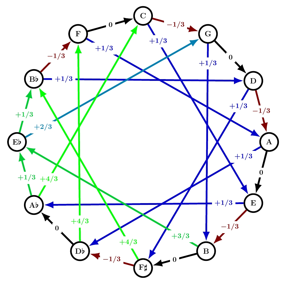
Werckmeister II

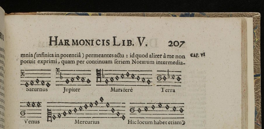
This is another name for quarter-comma meantone. Quarter-comma meantone was extremely popular from about 1550 until around 1690, when well temperaments started taking over. I discussed it extensively starting here, but remember:

All but one of the fifths are 1/4 comma flat, making the thirds built from those fifths ‘just’, with frequency ratios of exactly 5/4: these are the black arrows labelled 0. Unfortunately, the sum of the numbers on the circle of fifths needs to be -1. This forces the remaining fifth to be 7/4 commas sharp: it’s a painfully out-of-tune ‘wolf fifth’. And the thirds that cross this fifth are forced to be even worse: 8/4 commas sharp. Those are the problems that Werckmeister sought to solve with his next tuning system!

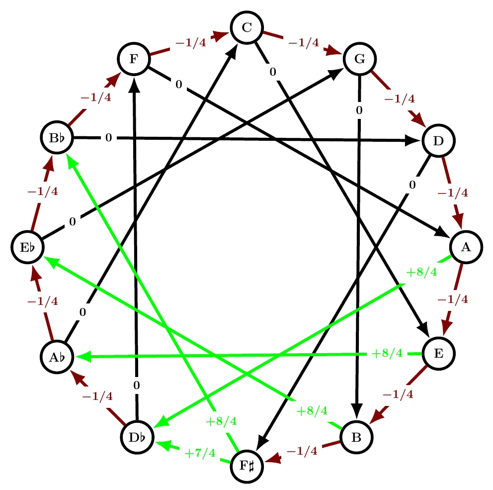
Werckmeister III

This was probably the world’s first well tempered tuning system! It’s definitely one of the most popular. Here it is:

4 of the fifths are 1/4 comma flat, so the total of the numbers around the circle is -1, as required by the laws of math, without needing any positive numbers. This means we don’t need any fifths to be sharp. That’s nice. But the subtlety of the system is the location of the flatted fifths: starting from C in the circle of fifths they are the 1st, 2nd, 3rd and… not the 4th, but the 6th!

I’ll talk about this more next time. For now, here’s a more elementary point. Comparing this system to quarter-comma meantone, you can see that it’s greatly smoothed down: instead of really great thirds in black and really terrible ones in garish fluorescent green, Werckmeister III has a gentle gradient of mellow hues. That’s ‘well temperament’ in a nutshell.

For more, see:

• Wikipedia, Werckmeister temperament III.

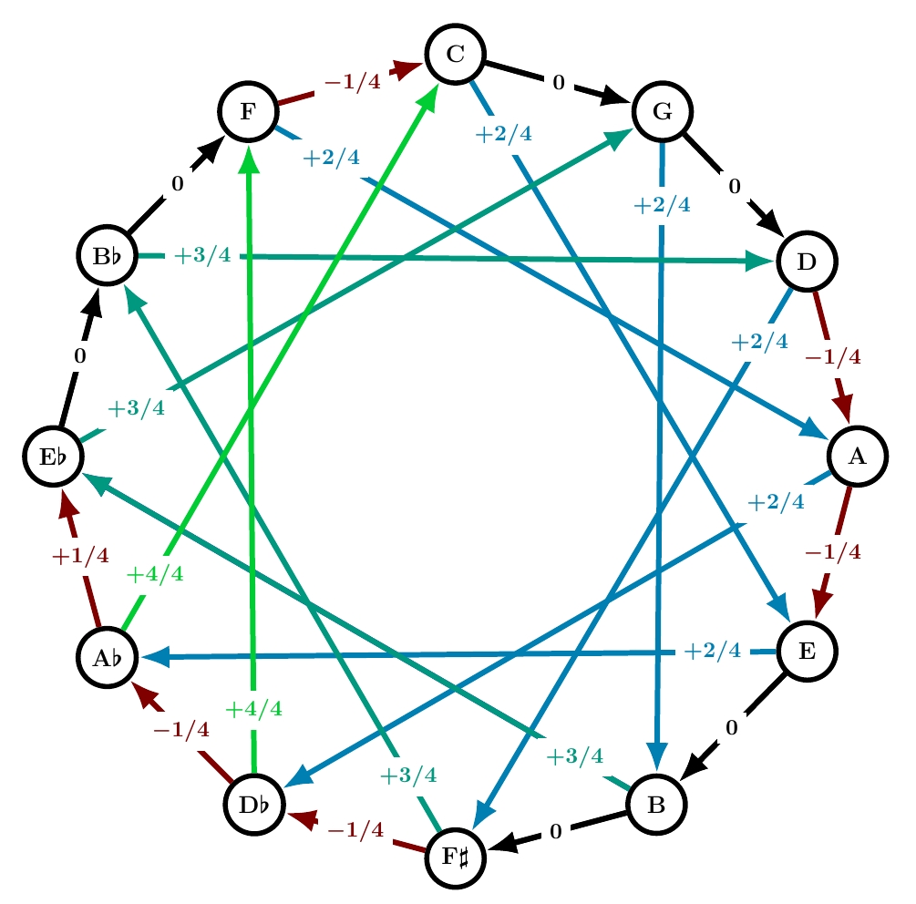
Werckmeister IV

This system is based not on 1/4 commas but on 1/3 commas!

As we go around the circle of fifths starting from B♭, every other fifth is 1/3 comma flat… for a while. But if we kept doing this around the whole circle, we’d get a total of -4. The total has to be -1. So we eventually need to compensate, and Werckmeister IV does so by making two fifths 1/3 comma sharp.

I will say more about Werckmeister IV in a post devoted to systems that use 1/3 and 1/6 commas. But you can already see that its color gradient is sharper than Werckmeister III. Probably as a consequence, it was never very popular.

For more, see:

• Wikipedia, Werckmeister temperament IV.

Werckmeister V

This is another system based on 1/4 commas:

Compared to Werckmeister III this has an extra fifth that’s a quarter comma flat—and thus, to compensate, a fifth that’s a quarter comma sharp. The location of the flat fifths seems a bit more random, but that’s probably just my ignorance.

For more, see:

• Wikipedia, Werckmeister temperament V.

Werckmeister VI

This system is based on a completely different principle. It also has another really cool-sounding name—the ‘septenarius tuning’—because it’s based on dividing a string into 196 = 7 × 7 × 4 equal parts. The resulting scale has only rational numbers as frequency ratios, unlike all the other well temperaments I’m discussing. Werckmeister described this system as “an additional temperament which has nothing at all to do with the divisions of the comma, nevertheless in practice so correct that one can be really satisfied with it”. For details, go here:

• Wikipedia, Werckmeister temperament VI.

Werckmeister on equal temperament

Werckmeister was way ahead of his time. He was not only the first, or one of the first, to systematically pursue well temperaments. He also was one of the first to embrace equal temperament! This system took over around 1790, and rules to this day. But Werckmeister advocated it much earlier—most notably in his final book, published in 1707, one year after his death.

There is an excellent article about this:

• Dietrich Bartel, Andreas Werckmeister’s final tuning: the path to equal temperament, Early Music 43 (2015), 503–512.

You can read it for free if you register for JSTOR. It’s so nice that I’ll quote the beginning:

Any discussion regarding Baroque keyboard tunings normally includes the assumption that Baroque musicians employed a variety of unequal temperaments, allowing them to play in all keys but with individual keys exhibiting unique characteristics, the more frequently used diatonic keys featuring purer 3rds than the less common chromatic ones. Figuring prominently in this discussion are Andreas Werckmeister’s various suggestions for tempered tuning, which he introduces in his Musicalische Temperatur. This is not Werckmeister’s last word on the subject. In fact, the Musicalische Temperatur is an early publication, and the following decade would see numerous further publications by him, a number of which speak on the subject of temperament.

Of particular interest in this regard are Hypomnemata Musica (in particular chapter 11), Die Nothwendigsten Anmerckungen (specifically the appendix in the undated second edition}, Erweiterte und verbesserte Orgel-Probe (in particular chapter 32), Harmonologia Musica (in particular paragraph 27) and Musicalische Paradoxal-Discourse (in particular chapters 13 and 23-5). Throughout these publications, Werckmeister increasingly championed equal temperament. Indeed, in his Paradoxal Discourse much of the discussion concerning other theoretical issues rests on the assumption of equal temperament. Also apparent is his increasing concern with theological speculation, resulting in a theological justification taking precedence over a musical one in his argument for equal temperament. This article traces Werckmeister’s path to equal temperament by examining his references to it in his publications and identifying the supporting arguments for his insistence on equal temperament.

In his Paradoxal Discourse, Werckmeister wrote:

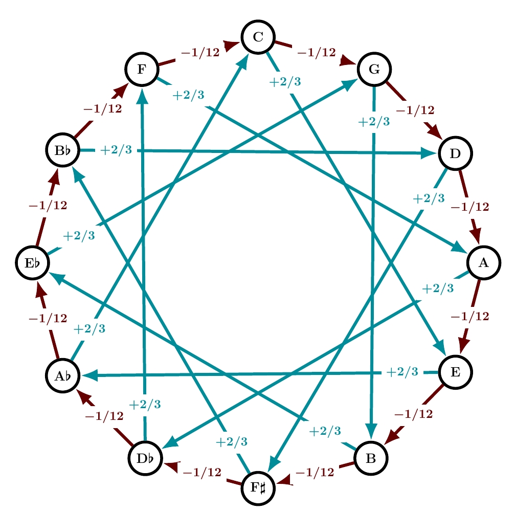
Some may no doubt be astonished that I now wish to institute a temperament in which all 5ths are tempered by 1/12, major 3rds by 2/3 and minor 3rds by 3/4 of a comma, resulting in all consonances possessing equal temperament, a tuning which I did not explicitly introduce in my Monochord.

This is indeed equal temperament:

And in a pun on ‘wolf fifth’, he makes an excuse for not talking about equal temperament earlier:

Had I straightaway assigned the 3rds of the diatonic genus, that tempering which would be demanded by a subdivision of the comma into twelve parts, I would have been completely torn apart by the wolves of ignorance. Therefore it is difficult to eradicate an error straightaway and at once.

However, it seems more likely to me that his position evolved over the years.

What’s next?

You are probably getting overwhelmed by the diversity of tuning systems. Me too! To deal with this, I need to compare similar systems. So, next time I will compare systems that are based on making a bunch of fifths a quarter comma flat. The time after that, I’ll compare systems that are based on making a bunch of fifths a third or a sixth of a comma flat.

---

For more on Pythagorean tuning, read this series:

• Pythagorean tuning.

For more on just intonation, read this series:

• Just intonation.

For more on quarter-comma meantone tuning, read this series:

• Quarter-comma meantone.

For more on well-tempered scales, read this series:

• Part 1. An introduction to well temperaments.

• Part 2. How small intervals in music arise naturally from products of integral powers of primes that are close to 1. The Pythagorean comma, the syntonic comma and the lesser diesis.

• Part 3. Kirnberger’s rational equal temperament. The schisma, the grad and the atom of Kirnberger.

• Part 4. The music theorist Kirnberger: his life, his personality, and a brief introduction to his three well temperaments.

• Part 5. Kirnberger’s three well temperaments: Kirnberger I, Kirnberger II and Kirnberger III.

For more on equal temperament, read this series:

• Equal temperament.

Agent-Based Models (Part 6)

Today I’d like to start explaining an approach to stochastic time evolution for ‘state charts’, a common approach to agent based models. This is ultimately supposed to interact well with Kris Brown’s cool ideas on formulating state charts using category theory. But one step at a time!

I’ll start with a very simple framework, too simple for what we need. Later I will make it fancier—unless my work today turns out to be on the wrong track.

Today I’ll describe the motion of agents through a graph, where each vertex of the graph represents a possible state. Later I’ll want to generalize this, replacing the graph by a Petri net. This will allow for interactions between agents.

Today the probability for an agent to hop from one vertex of the graph to another by going along some edge will be determined the moment the agent arrives at that vertex. It will depend only on the agent and the various edges leaving that vertex. Later I’ll want this probability to depend on other things too—like whether other agents are at some vertex or other. When we do that, we’ll need to keep updating this probability as the other agents move around.

Okay, let’s start.

We begin with a finite graph of the sort category theorists like, sometimes called a ‘quiver’. Namely:

• a finite set of vertices or states,

• a finite set of edges or transitions,

• maps mapping each edge to its source and target, also called its upstream and downstream.

Then we choose

• a finite set of agents.

Our model needs one more ingredient, a stochastic map called the jump function , which I will describe later. But let’s start talking about how we ‘run’ the model.

At each moment in time there will be a state map

saying what vertex each agent is at. Note, I am leaving the time-dependence of implicit here! We could call it if we want, but I think that will ultimately more confusing than helpful. I prefer to think of as a kind of ‘database’ that we will keep updating as time goes on.

Regardless, our main goal is to describe how this map changes with time: given initially we want our software to compute it for later times. But this computation will be stochastic, not deterministic. Practically speaking, this means we’ll use (pseudo)random number generators as part of this computation.

We could subdivide the real line into lots of little ‘time steps’ and do a calculation at each time step to figure out what each agent will do at that step: that’s called incremental time progression. But that’s computationally expensive.

So instead, we’ll use a version of discrete event simulation. We only keep track of events: times when an agent jumps from one state to another. Between events, nothing happens, so our simulation can jump directly from one event to the next.

So, whenever an event happens, we just need to compute the time at which the next event happens, and what actually happens then: that is, which agent moves from the state it’s in to some other state, and what that other state is.

For this we need to think about what the agents can do. For each vertex there is a set of edges going from that vertex to other vertices. An agent at vertex can move along any of these edges and reach a new vertex. So these are the questions we need to answer about this agent:

• which edge will it move along?

and

• when will it do this?

We will answer these questions stochastically, and we will do it by fixing a stochastic map called the jump function:

Briefly, tells us the time for a specific agent to make a specific transition if it arrived at the state upstream to that transition at a specific time.

The squiggly arrow means that is not an ordinary map, but rather a stochastic map. Mathematically, this means it maps points in to probability distributions on In practice, a stochastic map is a map whose value depends not only on the inputs to that map, but also on a random number generator.

Suppose is an agent, is an edge of our graph, and is a time. Then is the answer to this question:

If at time agent arrives at the vertex when will this agent move along the edge to the vertex given that it doesn’t do anything else first?

Here’s what we do with this information. At every moment in time we keep track of some information about each agent namely:

• Which vertex is it at now? This is

• For each edge whose upstream is when will agent move along this edge if it doesn’t do anything else first? Call this time

I need to explain how we compute these. Let’s assume that at some moment in time an agent has just moved along some edge. More specifically, suppose agent has just moved to some vertex At this moment we update the following information:

1) We set

(So, we update the state of the agent.)

2) For every edge with we set

(So, we update our table of times at which agent will move along each available edge, given that it doesn’t do anything else first.)

Now we need to compute the next time at which something happens, namely And we need to compute what actually happens then!

To do this, we look through our table of times for all agents and all edges with and see which time is smallest. If there’s a tie, break it by adding a little bit to some times Then let be the agent-edge pair that minimizes

3) We set

Then here’s what we do at time We take the state of agent and update it, to indicate that it’s moved along the edge More precisely:

4) We set

And now we go back to step 1), and keep repeating this loop.

Conclusion

As you can see, I’ve spent most of my time describing an algorithm. But my goal was really to figure out what data we need to describe an agent-based model of this specific sort. And I’ve seen that we need:

• a graph of states and transitions

• a set of agents

• a stochastic map describing the time for a specific agent to make a specific transition if it arrived in the state upstream to that transition at a specific time… and nothing else happens first.

Note that this last item gives us great flexibility. We can describe continuous-time Markov chains and also their semi-Markov generalization where the hazard rate of an edge (the probability per time for an agent to jump along that edge, assuming it doesn’t do anything else first) depends on how long the agent has resided in the upstream vertex. But we can also make these hazard rates have explicit time-dependence, and they can also depend on the agent!

Well Temperaments (Part 5)

Okay, let’s study Kirnberger’s three well-tempered tuning systems! I introduced them last time, but now I’ve developed a new method for drawing tuning systems, which should help us understand them better.

As we’ve seen, tuning theory involves two numbers close to 1, called the Pythagorean comma (≈ 1.0136) and the syntonic comma (= 1.0125). While they’re not equal, they’re so close that practical musicians often don’t bother to distinguish them! They call both a comma.

So, my new drawing style won’t distinguish the two kinds of comma.

Being a mathematician, I would like to say a lot about why we can get away with this. But that would tend to undercut my claim that the relaxed approach makes things simpler! I don’t want to be like the teacher who prefaces the explanation of a cute labor-saving trick with a long and confusing theoretical discussion of when it’s justified. So let me start by just diving in and using this new approach.

First I’ll illustrate this new approach with some tuning systems I’ve already discussed. Then I’ll show you Kirnberger’s three well-tempered systems. At that point you should be in a good position to make up your own well temperaments!

Pythagorean tuning

Here is Pythagorean tuning in my new drawing style:

The circle here is the circle of fifths. Most of these fifths are black arrows labeled by +0. These go between notes that have a frequency ratio of exactly 3/2. This frequency ratio gives the nicest sounding fifth: the Pythagorean fifth.

But one arrow on the circle is red, and labeled by -1. This fifth is one comma flat compared to a Pythagorean fifth. In other words, the frequency ratio of this fifth is 3/2 divided by a comma. This arrow is red because it’s flat—and it’s a fairly bright red because one comma flat is actually quite a lot: this fifth sounds pretty bad!

(The comma here is a Pythagorean comma, but never mind.)

This illustrates a rule that holds for every tuning system we’ll consider:

Rule 1. The numbers labeling arrows on the circle of fifths must sum to -1.

Now let’s look at Pythagorean tuning again, this time focusing on the arrows inside the circle of fifths:

The arrows inside the circle are major thirds. A few of them are black and labeled +0. These go between notes that have a frequency ratio of exactly 5/4. That’s the nicest sounding major third: the just major third.

But a some the arrows inside the circle are green, and labeled by +1. These major thirds are one comma sharp compared to the just major third. In other words, the frequency ratio between notes connected by these arrows is 5/4 times a comma. These arrows are green because they’re sharp—and it’s a fairly bright green because one comma sharp is actually quite a lot.

(These commas are syntonic commas, but never mind.)

Why do the major thirds work this way? It’s forced by the other rule governing all the tuning systems we’ll talk about:

Rule 2. The sum of the numbers labeling arrows for any four consecutive fifths, plus 1, equals the number labeling the arrow for the corresponding major third.

This rule creates an inherent tension in tuning systems! To get major thirds that sound really nice, not too sharp, we need some fifths to be flat. Pythagorean tuning is one way this tension can play out.

Equal temperament

Now let’s look at another tuning system: equal temperament.

Pythagorean tuning had eleven fifths that are exactly right, and one that’s 1 comma flat. The flatness was as concentrated as possible! Equal temperament takes the opposite approach: the flatness is spread out equally among all twelve fifths. Rule 1 must still hold: the total flatness of all the fifths is still 1 comma. So each fifth is 1/12 of a comma flat.

How does this affect the major thirds? Rule 2 says that each major third must be 2/3 of a comma sharp, since

2/3 = – 1/12 – 1/12 – 1/12 – 1/12 + 1

My pictures follow some color rules that are too boring to explain in detail, but bright colors indicate danger: intervals that are extremely flat or extremely sharp. In equal temperament the fifths are all reddish because they’re all flat—but it’s a very dark red, almost black, because they’re only slightly flat. The major thirds are fairly sharp, so their blue-green color is more noticeable.

Quarter-comma meantone

Now let’s look at another important tuning system: quarter-comma meantone. This system was very popular from 1550 until around 1690. Then people started inventing well temperaments as a reaction to its defects. So we need to understand it well.

Here it is:

All but one of the fifths are slightly flat: 1/4 comma flat. This is done to create a lot of just major thirds, since Rule 2 says

0 = -1/4 – 1/4 – 1/4 – 1/4 + 1

This is the beauty of quarter-comma meantone! But it’s obtained at a heavy cost, as we can see from the glaring fluorescent green.

Because 11 of the fifths are 1/4 comma flat, the remaining one must be a whopping 7/4 commas sharp, by Rule 1:

7/4 + 11 × -1/4 = -1

This is the famous ‘wolf fifth’. And by Rule 2, this wolf fifth makes the major thirds near it 2 commas sharp, since

2 = 7/4 – 1/4 – 1/4 – 1/4 + 1

In my picture I wrote ‘8/4’ instead of 2 because I felt like keeping track of quarter commas.

The colors in the picture should vividly convey the ‘extreme’ nature of quarter-comma meantone. As long as you restrict yourself to playing the dark red fifths and black major thirds, it sounds magnificently sweet. But as soon as you enter the fluorescent green region, it sounds wretched! Well temperaments were created to smooth this system down… without going all the way to the bland homogeneity of equal temperament.

And now let’s look at Kirnberger’s three well tempered systems. Only the third was considered successful, and we’ll see why.

Kirnberger I

Here is Kirnberger I:

The flatness of the fifths is concentrated in a single fifth, just as in Pythagorean tuning. Indeed, from this picture Kirnberger I looks just like a rotated version of Pythagorean tuning! That’s a bit deceptive, because in Kirnberger I the flat fifth is flat by a syntonic rather than a Pythagorean comma. But this is precisely the sort of nuance my new drawing style ignores. And that’s okay, because the difference between the syntonic and Pythagorean comma is inaudible.

So the only noticeable difference between Kirnberger I and Pythagorean tuning is the location of flat fifth. And it’s hard to see any advantage of putting it so close to C as Kirnberger did, rather than putting it as far away as possible.

Thus, it’s not so suprising that I’ve never heard of anyone actually using Kirnberger I. Indeed it’s rare to even see a description of it: it’s very obscure compared to Kirnberger II and Kirnberger III. Luckily it’s on Wikipedia:

• Wikipedia, Kirnberger temperament.

Kirnberger II

Here is Kirnberger’s second attempt:

This time instead of a single fifth that’s 1 comma flat, he used two fifths that are 1/2 comma flat.

As a result, only 3 major thirds are just, as compared to 4 in Kirnberger I. But the number of major thirds that are 1 comma sharp has gone down from 8 to 7. The are also 2 major thirds that are 1/2 comma sharp—the bluish ones. So, this system is less ‘extreme’ than Kirnberger I: the pain of sharp major thirds is more evenly distributed. As a result, this system was more widely used. But it was never as popular as Kirnberger III.

For more, see:

• Carey Beebe, Technical Library: Kirnberger II.

Kirnberger III

Here is Kirnberger’s third and final try:

This time instead of a two fifths that are 1/2 comma flat, he used four fifths that are 1/4 comma flat! A very systematic fellow.

This system has only one just major third. It has 2 that are 1/4 comma sharp, 2 that are 2/4 comma sharp, 2 that are 3/4 comma sharp, and only 3 that are 1 comma sharp. So it’s noticeably less ‘extreme’ than Kirnberger II: fewer thirds that are just, but also fewer that are painfully sharp.

I think you really need to stare at the picture for a while, and think about how Rule 2 plays out, to see the beauty of Kirnberger III. But the patterns become a bit more visible if we rotate this tuning system to give it bilateral symmetry across the vertical axis, and write the numbers in a symmetrical way too:

Rotating a tuning system just means we’re starting it at a different note—‘transposing’ it, in music terminology.

The harpsichord tuning expert Cary Beebe writes:

One of the easiest—and most practical—temperaments to set dates from 1779 and is known as Kirnberger III. For a while, some people thought that this might be Bach’s temperament, seeing as Johann Philipp Kirnberger (1721–1783) learnt from the great JS himself. Despite what you might have been taught, Bach neither invented nor used Equal Temperament. He probably used many different tuning systems—and if he had one particular one in mind for any of his works, he never chose to write clear directions for setting it. Note that his great opus is called the Well-tempered Clavier in English, not the “Equal Tempered Clavichord”, as it has too often been mistranslated. You will find several other Bach temperaments discussed later in this series.

There are other commas to learn, and a whole load of other technical guff if you really want to get into this quagmire, but here you will forgive me if we regard the syntonic comma as for all practical purposes the same size as the Pythagorean. After all, don’t you just want to tune your harpsichord instead of go for a science degree?

Here’s how you go about setting Kirnberger III…

Then he explains how to tune a harpischord in this system:

• Carey Beebe, Technical Library: Kirnberger III.

Carey Beebe is my hero these days, because he explains well temperaments better than anyone else I’ve found. My new style of drawing tuning systems is inspired by his, though I’ve added some extra twists like drawing all the major thirds, and using colors.

Technical details

If you’re wondering what Beebe and I mean about Pythagorean versus syntonic commas, here you can see it. Here is Kirnberger I drawn in my old style, where I only drew major thirds that are just, and I drew them in dark blue:

Kirnberger I has one fifth that’s flat by a factor of the syntonic comma:

σ = 2^-4 · 3⁴ · 5^-1 = 81/80 = 1.0125

But as we go all the way around the circle of fifths the ‘total flatness’ must equal the Pythagorean comma:

p = 2^-19 · 3¹² = 531441/524288 ≈ 1.013643

That’s just a law of math. So Kirnberger compensated by having one fifth that’s flat by a factor of p/σ, which is called the ‘schisma’:

χ = p/σ = 2^-15 · 5 · 3⁸ = 32805/32768 ≈ 1.001129

He stuck this ‘schismatic fifth’ next to the tritone, since that’s a traditional dumping ground for annoying glitches in music. But it barely matters since the schisma is so small.

(That said, the schisma is almost precisely 1/12th of a Pythagorean comma, or more precisely p^1/12—a remarkable coincidence discovered by Kirnberger, which I explained in Part 3. And I did draw the 1/12th commas in equal temperament! So you may wonder why I didn’t draw the schisma in Kirnberger I. The answer is simply that in both cases my decision was forced by rules 1 and 2.)

Here’s Kirnberger II in a similar style:

Here the schismatic fifth compensates for using two 1/2 commas that are syntonic rather than Pythagorean.

And here’s Kirnberger III:

Now the schismatic fifth compensates for using four 1/4 commas that are syntonic rather than Pythagorean.

---

For more on Pythagorean tuning, read this series:

• Pythagorean tuning.

For more on just intonation, read this series:

• Just intonation.

For more on quarter-comma meantone tuning, read this series:

• Quarter-comma meantone.

For more on well-tempered scales, read this series:

• Part 1. An introduction to well temperaments.

• Part 2. How small intervals in music arise naturally from products of integral powers of primes that are close to 1. The Pythagorean comma, the syntonic comma and the lesser diesis.

• Part 3. Kirnberger’s rational equal temperament. The schisma, the grad and the atom of Kirnberger.

• Part 4. The music theorist Kirnberger: his life, his personality, and a brief introduction to his three well temperaments.

• Part 5. Kirnberger’s three well temperaments: Kirnberger I, Kirnberger II and Kirnberger III.

For more on equal temperament, read this series:

• Equal temperament.