Today I’d like to start explaining an approach to stochastic time evolution for ‘state charts’, a common approach to agent based models. This is ultimately supposed to interact well with Kris Brown’s cool ideas on formulating state charts using category theory. But one step at a time!
I’ll start with a very simple framework, too simple for what we need. Later I will make it fancier—unless my work today turns out to be on the wrong track.
Today I’ll describe the motion of agents through a graph, where each vertex of the graph represents a possible state. Later I’ll want to generalize this, replacing the graph by a Petri net. This will allow for interactions between agents.
Today the probability for an agent to hop from one vertex of the graph to another by going along some edge will be determined the moment the agent arrives at that vertex. It will depend only on the agent and the various edges leaving that vertex. Later I’ll want this probability to depend on other things too—like whether other agents are at some vertex or other. When we do that, we’ll need to keep updating this probability as the other agents move around.
Okay, let’s start.
We begin with a finite graph of the sort category theorists like, sometimes called a ‘quiver’. Namely:
• a finite set 
• a finite set 
• maps 
Then we choose
• a finite set 
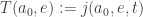
Our model needs one more ingredient, a stochastic map called the jump function 
At each moment in time 

saying what vertex each agent is at. Note, I am leaving the time-dependence of 

Regardless, our main goal is to describe how this map
We could subdivide the real line 
So instead, we’ll use a version of discrete event simulation. We only keep track of events: times when an agent jumps from one state to another. Between events, nothing happens, so our simulation can jump directly from one event to the next.
So, whenever an event happens, we just need to compute the time at which the next event happens, and what actually happens then: that is, which agent moves from the state it’s in to some other state, and what that other state is.
For this we need to think about what the agents can do. For each vertex 


• which edge will it move along?
and
• when will it do this?
We will answer these questions stochastically, and we will do it by fixing a stochastic map called the jump function:
Briefly,
The squiggly arrow means that 

Suppose 


If at time
agent
when will this agent move along the edge
to the vertex
given that it doesn’t do anything else first?
Here’s what we do with this information. At every moment in time we keep track of some information about each agent 
• Which vertex is it at now? This is

• For each edge 
I need to explain how we compute these. Let’s assume that at some moment in time 


1) We set

(So, we update the state of the agent.)
2) For every edge 
(So, we update our table of times at which agent
Now we need to compute the next time at which something happens, namely 
To do this, we look through our table of times 


3) We set

Then here’s what we do at time 


4) We set

And now we go back to step 1), and keep repeating this loop.
Conclusion
As you can see, I’ve spent most of my time describing an algorithm. But my goal was really to figure out what data we need to describe an agent-based model of this specific sort. And I’ve seen that we need:
• a graph 
• a set
• a stochastic map 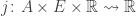
Note that this last item gives us great flexibility. We can describe continuous-time Markov chains and also their semi-Markov generalization where the hazard rate of an edge (the probability per time for an agent to jump along that edge, assuming it doesn’t do anything else first) depends on how long the agent has resided in the upstream vertex. But we can also make these hazard rates have explicit time-dependence, and they can also depend on the agent!


The state chart paradigm sounds like a finite state machine, especially if we assume that the map is deterministic. So is it possible to view them as a model of computation, and is it Turing complete? This would give some indication of how generally powerful this paradigm is.
BTW in the stochastic case, are the individual “uses” of all assumed to be stochastically independent?
I don’t really want the paradigm to be computationally powerful; I’m just hoping it will conveniently capture a certain interesting class of multi-agent (or you could say ‘multi-particle) stochastic processes. And it’s leaving out one of the most important features I’ll need to include later, namely interactions between agents. I was going to include those features, but I got caught up trying to work out the details of discrete event simulation, because I’ve never thought about it much and it’s quite different from the ODE-based outlook I’m more used to.
However, the perspective of computational power could be interesting too! Suppose is deterministic.
1) If is independent of the agent
  and the time
  we have a deterministic finite state machine. Any agent
  arriving at some state at time
  jumps along the edge leaving that state that minimizes
Finite state machines are far from Turing complete, right?
2) If we allow to depend on the agent
  but not
  we have a collection of finite state machines, one for each agent.
3) If we allow to depend on
  but not
  we get something I haven’t heard about so much: a kind of finite state machine whose transition rules can change with time!
Tobias wrote:
Yes! Otherwise we’d be injecting correlations into our model that act a bit like “spooky action at a distance”, e.g. in an extreme case the probability that each person catches a cold is 50% but we either all get a cold or none of us does.
Right, it makes sense that the individual uses of would be independent across agents. But how about the different uses for one and the same agent in the same state? When I’m in a healthy state, then there could be reasons for why the times that it takes for me to catch a cold, the flu or covid are correlated, because there can be confounding factors, for example because I’m taking the tram one day and it’s packed, which makes it more likely that I’ll catch some bug. But presumably the idea is that all such confounders are considered part of the state?
We still want different instances of to be uncorrelated, because we don’t want to hide correlations in the black box of this
  function: if we want correlations, we want them to be easily visible in the model… and I mean literally visible.
In the simple framework I’m describing, the confounders you mention should be considered part of the state. But the framework I’m using is well-known to create a problem: there’s a combinatorial explosion of states. E.g. if we have 10 health states and 10 employment states and 10 location states and 10 interpersonal relationship states, we’re already getting a graph with 1000 vertices—which is bad because modelers actually want to work with these graphs visually using graphical user interfaces.
One common solution is that instead of drawing a single graph that’s a product of several different graphs, we just draw those several different graphs—e.g. a health graph and an employment graph and a location graph and an interpersonal relationship graph. Each graph represents a different ‘aspect’ of the agent’s state. Then we represent different aspects of our agent as moving from state to state in each one of those graphs.
But then we need to describe the interaction between these different aspects using something like ‘informational links’ between graphs: otherwise we’d just have uncorrelated evolution of each aspect of state. So that’s one of the next steps I want to take.
All of this so far is mainly formalizing and generalizing what actual epidemiologists already do with agent-based models. Our team is not wanting to change these practices so radically that epidemiologists won’t use our software! But my trick in this post of having multiple agents move around in the same graph, instead of having separate graphs for each agent, appears to be new. At least it was new to Nate Osgood, who is my main ‘native informant’ about the practice of agent-based modeling in epidemiology!
There’s a programming language called Ada that has multi-threading built-in (the equivalent of agents are declared using the Task keyword). Petri Net semantics are built-in using rendezvous semantics, inspired by Tony Hoare’s Communicating Sequential Processes model, Ada is a real-time programming language, so making it into a Discrete Event Simulation is difficult. Fortunately there was a version of Ada called GNAT built on GNU. So I took the real-time Ada runtime and replaced it with a Discrete Event Engine, mainly a FIFO scheduler, and got it to work. This was published in a couple of articles, calling the system linked library DEGAS
Ludwig, Luke, and Paul Pukite. “DEGAS: discrete event Gnu advanced scheduler.” Proceedings of the 2006 annual ACM SIGAda international conference on Ada. 2006.
Pukite, Paul, and Luke Ludwig. “Generic discrete event simulations using DEGAS: application to logic design and digital signal processing.” Proceedings of the 2007 ACM international conference on SIGAda annual international conference. 2007.
It was pretty cool, as we used it for testing robotic simulations. A real-time application that may run for hours or days, can run in seconds because of the way that the event schedule can be compressed. It also could be used in a way similar to VHDL.
Thinking about this is sad though because I only recently found out that my colleague working with me on this project, Luke Ludwig, had died in a plane accident, along with his wife, both at the age of 42. After I worked with him, he had gone on to be the chief software engineer for a startup sports/team scheduling company called SportEngine. I’d say that likely millions of kids have indirectly used the application in playing team competitive sports, and the software is now owned by NBC. Hope his two young children realize what a talent he had, and to think that he went from a research tool used by a handful of us on to greater things is bittersweet.
Yes, we used the SportsEngine app to follow tournament standings when my daughter was playing middle-school basketball. I never really thought about the math behind it; I just knew that we got updates faster than we could by waiting for the officials to post them.
That seems pretty vague. But if all of the probability distributions are continuous, then this will only ever happen with probability 0.
Since time will probably be modeled in software using finite-precision floating-point numbers, the chance of a tie is nonzero… but usually small. According to Nate Osgood this is considered acceptable in agent-based modeling. Since we’re using stochastic models anyway, a little extra ‘tie-breaking noise’ shouldn’t really hurt the conclusions we draw. Or to put it another way: if it does, something is probably wrong with how we’re using these models.
It seems weird to break the tie by adding some time rather than by flipping a (virtual) coin, but as long as you flip a coin to decide which one to add the time to, then it comes out the same either way.
In reality I will let the people who write the software deal with this issue; I mainly just wanted to admit that it’s an issue.
One of the great advantages of replacing a real-time software runtime with a discrete event engine (as my comment upthread describes) is that it becomes exactly deterministic. Each time it runs, it will give the same result — while a wall-clock will always add some sort of time jitter, making the real-time results non-deterministic. This has many benefits for regression testing and formal analysis. That’s why all digital integrated circuits are designed with a language that supports both logic design and discrete-event simulation, see VHDL, Verilog, and higher-level library component languages that build on C or C++.
As to breaking a tie in this scenario, the rule would be the first added to the queue would be the tie-breaker. That would maintain determinism. For a stochastically stimulated and event-triggered run, this would be less important.
Nice! I’m glad someone has thought about this more than I have.