Last time we saw clues that stochastic Petri nets are a lot like quantum field theory, but with probabilities replacing amplitudes. There’s a powerful analogy at work here, which can help us a lot. So, this time I want to make that analogy precise.
But first, let me quickly sketch why it could be worthwhile.
A Poisson process
Consider this stochastic Petri net with rate constant 

It describes an inexhaustible supply of fish swimming down a river, and getting caught when they run into a fisherman’s net. In any short time 


Problem. Suppose we start out knowing for sure there are no fish in the fisherman’s net. What’s the probability that he has caught 

At any time there will be some probability of having caught 

Here 

This describes how the probability of having caught any given number of fish changes with time.
What’s the operator 

We can try to apply this to our fish. If at some time we’re 100% sure we have

so applying the creation operator gives

One more fish! That’s good. So, an obvious wild guess is

where
If you know how to exponentiate operators, you know to solve this equation:
It’s easy:
Since we start out knowing there are no fish in the net, we have

so with our guess for
But 


So, if our guess is right, the probability of having caught

Unfortunately, this can’t be right, because these probabilities don’t sum to 1! Instead their sum is

We can try to wriggle out of the mess we’re in by dividing our answer by this fudge factor. It sounds like a desperate measure, but we’ve got to try something!
This amounts to guessing that the probability of having caught

And this is right! This is called the Poisson distribution: it’s famous for being precisely the answer to the problem we’re facing.
So on the one hand our wild guess about

The extra 
So, a wild guess corrected by an ad hoc procedure seems to have worked! But what’s really going on?
What’s really going on is that 

In quantum theory, self-adjoint Hamiltonians are okay. But in probability theory, we need some other kind of Hamiltonian. Let’s figure it out.
Probability versus quantum theory
Suppose we have a system of any kind: physical, chemical, biological, economic, whatever. The system can be in different states. In the simplest sort of model, we say there’s some set 
• In a probabilistic model, we may instead say that the system has a probability 


• In a quantum model, we may instead say that the system has an amplitude

Probabilities and amplitudes are similar yet strangely different. Of course given an amplitude we can get a probability by taking its absolute value and squaring it. This is a vital bridge from quantum theory to probability theory. Today, however, I don’t want to focus on the bridges, but rather the parallels between these theories.
We often want to replace the sums above by integrals. For that we need to replace our set
• In a probabilistic model, the system has a probability distribution 

• In a quantum model, the system has a wavefunction 

In probability theory, we integrate 


We don’t need to think about sums over sets and integrals over measure spaces separately: there’s a way to make any set
In short, integrals are more general than sums! So, I’ll mainly talk about integrals, until the very end.
In probability theory, we want our probability distributions to be vectors in some vector space. Ditto for wave functions in quantum theory! So, we make up some vector spaces:
• In probability theory, the probability distribution

• In quantum theory, the wavefunction

You may wonder why I defined 
Now:
• The main thing we can do with elements of

• The main thing we can with elements of 

This gives a map that’s linear in one slot and conjugate-linear in the other:

First came probability theory with 


Stochastic versus unitary operators
Now let’s think about time evolution:
• In probability theory, the passage of time is described by a map sending probability distributions to probability distributions. This is described using a stochastic operator

meaning a linear operator such that

and

• In quantum theory the passage of time is described by a map sending wavefunction to wavefunctions. This is described using an isometry

meaning a linear operator such that

In quantum theory we usually want time evolution to be reversible, so we focus on isometries that have inverses: these are called unitary operators. In probability theory we often consider stochastic operators that are not invertible.
Infinitesimal stochastic versus self-adjoint operators
Sometimes it’s nice to think of time coming in discrete steps. But in theories where we treat time as continuous, to describe time evolution we usually need to solve a differential equation. This is true in both probability theory and quantum theory:
• In probability theory we often describe time evolution using a differential equation called the master equation:
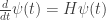
whose solution is

• In quantum theory we often describe time evolution using a differential equation called Schrödinger’s equation:
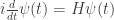
whose solution is
In fact the appearance of 
Let’s guess what properties an operator 

Then we differentiate this with respect to 

or in other words

Physicists call an operator obeying this condition self-adjoint. Mathematicians know there’s more to it, but today is not the day to discuss such subtleties, intriguing though they be. All that matters now is that there is, indeed, a correspondence between self-adjoint operators and well-behaved ‘one-parameter unitary groups’
But now let’s copy this argument to guess what properties an operator

and

We can differentiate the first equation with respect to

for all
But what about the second condition,

It seems easier to deal with this in the special case when integrals over
In this case, 

As a warmup, let’s see what it means for an operator
to be stochastic in this case. We’ll take the conditions
and
and rewrite them using matrices. For both, it’s enough to consider the case where 
In these terms, the first condition says

for each column 

for all 
Next, let’s see what we need for an operator 

and work to first order in

which requires

Saying that each entry is nonnegative amounts to

When 
So, let’s say
I don’t love this terminology: do you know a better one? There should be some standard term. People here say they’ve seen the term ‘stochastic Hamiltonian’. The idea behind my term is that any infintesimal stochastic operator should be the infinitesimal generator of a stochastic process.
In other words, when we get the details straightened out, any 1-parameter family of stochastic operators

obeying


and continuity:

should be of the form
for a unique ‘infinitesimal stochastic operator’
When
Luckily, for our work on stochastic Petri nets, we only need to understand the case where
The moral
Now we can see why a Hamiltonian like 
In this example, our set of states is the natural numbers:

The probability distribution

tells us the probability of having caught any specific number of fish.
The creation operator is not infinitesimal stochastic: in fact, it’s stochastic! Why? Well, when we apply the creation operator, what was the probability of having 
Using our fancy abstract notation, these conditions say:

and
So, precisely by virtue of being stochastic, the creation operator fails to be infinitesimal stochastic:

Thus it’s a bad Hamiltonian for our stochastic Petri net.
On the other hand,

precisely because
You may be thinking: all this fancy math just to understand a single stochastic Petri net, the simplest one of all!
But next time I’ll explain a general recipe which will let you write down the Hamiltonian for any stochastic Petri net. The lessons we’ve learned today will make this much easier. And pondering the analogy between probability theory and quantum theory will also be good for our bigger project of unifying the applications of network diagrams to dozens of different subjects.


should be
And you have a ‘the the’ somewhere.
Thanks! I’ll fix those!
By the way, I was expecting you to say “we’re not just changing from to
to  when we go from quantum theory to probability theory: we’re also changing the rig of scalars from
  to the nonnegative reals”. That’s why I muttered:
I just didn’t feel like getting into ‘rigs’ in this supposedly more ‘practical’ article.
Yep. And then there’s your observation that the normalization of distributions can be captured with Durov’s generalized rings.
Oh, there’s another for
for  change needed after “This is described using an isometry…”
Thanks, fixed.
Yes, it would be very nice to polish all the math to a glossy sheen using category theory. But in my new persona, I want to focus more on insights that are lurking in various different kinds of applied work, using math as needed to take insights from specific subjects and apply them more generally, without sailing so high into the abstractosphere that only mathematicians and particle physicists pay attention.
This is part of the ‘green mathematics’ dream: a kind of math where you don’t need to build an enormous particle accelerator to get good ideas from the physical world.
For example, the literature on chemical reaction networks is full of astounding ideas that deserve to be stated in a way non-chemists can appreciate, because they’re not particularly about chemistry. That’s one direction I want to head soon.
But you surely hold that category theory isn’t just for buffing up some mathematics to make it shine, but also for locating and analogizing insights from specific subjects. Of course the abstract methods used in the process can be kept hidden from sight.
David wrote:
Right, my remark came across as overly dismissive, but that’s a sign of internal struggle: I’m fighting against my desire to keep making the analogy between quantum theories and probabilistic theories nicer and nicer using more and more math. Making the analogies nicer is not just cosmetic: it’s important for digger deeper into what’s really going on, which after all is very mysterious. If the difference between probability theory and quantum theory were really just one between and
and  , you’d have to see what
  could do for you… but I really doubt that’s the way to go (though somebody should try). We could dig a bit deeper by thinking about commutative versus noncommutative C*-algebras, or perhaps matrix mechanics over different rigs…
However, all this would take me in a different direction than I’m trying to go. I want to work through lots of applications of ‘diagrams’ and ‘networks’ in different fields—population biology, systems ecology, chemistry and biochemistry, genomics, queuing theory, statistical inference and machine learning, and so on—and fit them together into a nice framework that’ll help people in any one field profit from the work in other fields. To do this I need help from people in all these different subjects. This makes me keenly aware that the benefits of fancy mathematics come with a painful cost: they limit the number of people who can join the conversation!
It’s very sad how the people who hold the most powerful tools in mathematics have become so isolated from the people who need them. Sad both for the people who need them, but also for those holding the tools.
I’ve got category theory in my bones by now, but it’s not as if I have notebooks full of category-theoretic reflections on diagrams and networks that I’m hiding from my readers here. Right now I’m mainly struggling to explain the relation between stochastic Petri nets, the chemical master equation and the Feynman diagram approach to quantum field theory.
Something’s a bit fishy here: are you sure you’re not producing about a Lapin process rather than a Poisson process? (Sorry, incredibly poor joke.)
The question that leaps up as someone who knows little about physics, does the kind of quantum theory that’s being used here model any kind of non-static equilibirum behaviours in physics (so that this modelling could eventually be used for general process modelling)? (So far nothing you’ve written is seems to be assuming equilibrium state.)
David wrote:
Yes!
More precisely: I’m setting up an analogy between probability theory and quantum theory, which then specializes to an analogy between stochastic Petri nets and the theory of Feynman diagrams.
Stochastic Petri nets are a very general tool for describing stochastic processes involving bunches of things of various kinds that can turn into other bunches of things. Feynman diagrams are a very general tool for describing quantum processes involving bunches of things of various kinds that turn into other bunches of things. The only really big differences are the differences I’ve described here: versus
  , stochastic operators versus unitary operators, etcetera. But these differences are so systematic that it’s easy to take wads of stuff from one theory and translate it over to the other—as I’ll soon explain.
In neither case is there any restriction to equilibrium states. Indeed, Feynman diagrams are most commonly used for computing the amplitude that two elementary particles will turn into something else when you smash them into each other in a particle accelerator—that’s about as far from equilibrium as you can get!
What if one tries to use square roots of measures. Wouldn’t that make it much closer to QM ?
You mean use square roots of finite measures instead of functions as a formulation of quantum mechanics? Yes, that would be fine. But then I’d want to use a space finite measures instead of
  with respect to a fixed measure… to keep the analogy nice. And I’m trying to avoid polishing the math to such a glossy shine that nobody but mathematicians can stand the glare.
  I’m mainly trying to generalize some quantum mechanics techniques (annihilation and creation operators, Feynman diagrams) to stochastic Petri nets, and here the measure space in question is always a countable set with counting measure. So, my more general remarks about measure spaces are already looking ahead a bit too far…
David wrote:
It’s got the seeds of a good joke in it. If Jacob and I ever write up these blog entries as more formal ‘lecture notes’, we’ll change ‘rabbit’ to ‘fish’ in the main example here, so that catching fish will be a Poisson process. As long as we don’t draw undue attention to that, it should be funny.
(I think puns are fun when they seem to arise effortlessly, but provoke groans when they require an obvious stretch. If so, the trick is to put a lot of work into the setup.)
The rabbits in this blog entry have now become fish.
John wrote:
I’d like to mention that this is a well known trick – the introduction of a generating function – and that there is a book called “generatingfunctionology” by Herbert Wilf free for download from the author’s webpage.
I love that stuff.
I taught a year-long course on generating functions and their use in quantum theory, starting here. The key idea was to think of generating functions as decategorified versions of ‘stuff types’. You could say what I’m doing now is warming up to apply some of the same ideas to classical probability theory.
In One-Parameter Semigroups of Positive Operators, Springer-Verlag, Berlin 1986, ISBN 978-3-540-16454-8 the authors investigate C0-semigroups on Banach lattices (e.g. ). Things are more complicated than in the Hilbert space situation and to get the desired characterization one most likely has to apply the standard Hille-Yosida generation theorem plus some condition on the resolvent depending on what exactly you mean by “stochastic”.
Thanks very much, I’ll check that out! Hille was my advisor’s advisor, so I’m always happy to use that theorem of his.
By chance today is one of the rare happy days when I made it to the math library…
For (un)bounded positive symmetric operators on
on  there are the 2 Beurling-Deny criteria, telling in terms of the quadratic form
  when
when  is positivity preserving resp.
  contractive. See M. Reed, B. Simon, Methods of Modern Math. Physics Vol. IV, Thm. XIII.50 resp. XIII.51 (p. 209-211). Both criteria can be amalgamated into one characterising
  generators of Markovian semigroups. This criterion is the cornerstone of the theory of “Dirichlet forms”, kind of generalizing Brownian motion on Riemannian manifolds to less smooth spaces. See M. Fukushima, Y. Oshima, M. Takeda, Dirichlet Forms and Symmetric Markov Processes, pp. 3-5.
This stuff is much related to Kato’s inequality (cf. Reed, Simon, Vol. II, Thm. X.27, p.183 and following pages for some real Schrödinger operator stuff). Also known as “diamagnetic inequality” (B. Simon) for magnetic Schrödinger stuff, or “semigroup domination” for estimations of Hodge heat flow in differential geometry.
Thanks a million, Florifulgurator!
I’m so glad you pointed out that Dirichlet forms are relevant here! I should have realized that. I first learned about Dirichlet forms when working on an earlier phase of my ‘networks’ project: electrical circuits made of resistors. But there I was mainly interested in Dirichlet forms on finite-dimensional vector spaces, so I had them filed in a different mental compartment than this ‘semigroups on ‘ business.
This could be a hint of something big: two different aspects of my networks project (electrical circuits made of resistors, and stochastic Petri nets) turn out to require the same math: Dirichlet forms.
Wow, now I think I see how they’re related! Stupidly, that had never occurred to me! This is exactly the sort of unification I’m looking for in this game. It keeps happening…
Here’s a bit about Dirichlet forms, from week297:
Stroock’s re/overview is superb. (Back then I was TA/RA in Germany. I handed it out as introductory reading for my seminar on Dirichlet forms.)
You mentioned a book Dirichlet Forms and Symmetric Markov Processes, and that reminded me: many of the Markov processes I’m interested in these days (e.g. those described by stochastic Petri nets) are nonsymmetric. Is there a good generalization of Dirichlet forms to handle those? Of course when working on a manifold we can consider Brownian motion plus drift, with the drift given by a vector field… but what if we’re just on an arbitrary measure space?
Oh yeah, I forgot about the symmetry question while happily browsing the old books again after a decade… – what is a “symmetric Petri net” … ?
I’ve never cared about the nonsymmetric case. But others did:
• Ma Z.M. and Röckner M.: Introduction to the Theory of (Non-Symmetric) Dirichlet Forms, Springer-Verlag, Berlin-Heidelberg-New York, 1992.
The field of generalized Dirichlet forms seems still quite active. Next time I’m at the library I’ll start catch up a little and first read this (or what google books hides of it): S. Albeverio, Theory of Dirichlet Forms and applications, in Lecture Notes in Math 1816 (Ecole d’été de probabilités de Saint-Flour XXX, 2000). Has a huge list of references on all kinds of variations of this theme.
Florifulgurator wrote:
Nice question! I’m not sure it’s a standard term, but it has an obvious meaning:
A symmetric Petri net is one where every transition is reversible.
A bit more precisely: for each transition with a given list of inputs and a given list of outputs, there’s a transition with those inputs as its outputs, and those outputs as its inputs. We call this other transition the reverse of the original transition.
More precisely still: a Petri net consists of a set of states, a set
  of transitions, and input and output functions
saying for each transition how many times each state appears as input or output. Every Petri net has a reversed Petri net where we switch the functions and
and  . A Petri net is symmetric if it’s isomorphic to its reversed version. Or, much better, if it’s equipped with an isomorphism to its reversed version. Then each transition has another transition called its reverse. Then we can define what it means for a stochastic Petri net to be symmetric: now the rate constant of each transition must equal that of its reverse.
Any stochastic Petri net gives rise to a Markov process. If the stochastic Petri net is symmetric, so is its Markov process.
Great! The wonderful thing about math is that there are tons of people working on tons of obscure-sounding subjects, so that when you get interested in something you usually find an entire book has been written about it already! Books that seem completely boring suddenly become fascinating when you need to know what’s in them.
I’ve been trying to unpick some of the notation (to figure out something that’s probably obvious if you’ve studied how this setup works for quantum physics). Here’s my understanding, in case it is in fact wrong. Firstly, lets change the “formal power series variable” used in the first section from to
to  just to be a bit clearer. The statement
is at this point viewing as a function of values
  in the space
  (not a function of time in this particular bit) into the complex numbers, which function must be non-negative for all arguments. Now I think that in this case the space is the discrete space
  , ie, powers of the formal variable. So while this is a statement about a function, it’s effectively a statement about individual coefficients in the formal power series that says that probabilities are non-negative. (This combined with the integral condition also gives probabilities must be at most 1.)
If I’m understanding correctly, means essentially coefficentOf(
 ), whilst
  denotes essentially replacing the formal variable
  with
with  , where
  is a new formal variable. (I’m used to generating functions and pgf’s, but analytic time varying pgf’s are new country to me.)
I see what’s confusing you. Your guesses look right. There’s a general situation and a particular situation here.
• In the general situation, we have a set of states . The probability distribution
  is a function assigning to each state
  a probability
  . Since probabilities are never negative, we have
  for all
  , or
, or
for short.
• In the particular situation, we’re talking about rabbits. Here is the set of natural numbers:
and the natural number means ‘the state of having caught
  rabbits’. In this particular situation, I wrote
  to mean the probability of having caught
  rabbits. And in this particular situation, I defined a power series in some formal variable
  —having nothing to do with the
  mentioned above!—whose coefficients are the probabilities
  . This is called a ‘generating function’. Just to confuse you further, I also called this generating function
  :
:
There is of course no need for this function to be nonnegative.
So, my use of and
and  was quite different in the general situation and the particular situation. I’m so used to rapidly switching between them that I never noticed how confusing it could be! I’ll fix this now.
I’ll guess that by ‘pgf’ you mean a ‘probability-generating function’, namely this thing:
Yes, this thing and everything else I’m calling will in general be a function of time as well.
Believe it or not, I’d never heard of ‘probability-generating functions’ before, though I’ve spent a lot of time on generating functions. Those who don’t know history are condemned to repeat it. So, thanks for pointing out that buzzword!
Okay, David, I’ve tried to make the article clearer. It was shocking to realize how incredibly confusing it would be to someone who couldn’t read my mind! Now:
• In the general situation we have a set of states and a probability distribution
  which assigns to each state
  a probability
  .
.
• In the particular situation of rabbits we have , and I write
  for the probability of having
  rabbits. I’m switching to the variable
  instead of
  here for purely traditional rather than conceptual reasons. I see the authors of Wikipedia article probability-generating function avoid this sentimental attitude: they use
  to stand for a natural number! Years of conditioning have made this unpalatable to me.
More importantly, starting from in this particular situation I define a probability-generating function
using a new letter to distinguish the variable here from any other variable, and a new font
  to distinguish the generating function from the probability distribution
  .
.
Thanks!
Thanks for clarifying things John. The article was actually already a very clear overview, it just required a little bit of effort to figure out the fine details. It’s a lot clearer in the fine details now.
I probably ought to point out for other people that part of my confusion was that in probability one often uses by looking at its various derivatives (which are related to the distribution’s moments) in
  so it is very much being viewed as a function, not just a neat way of writing an inifinite vector, which is why I initially thought that interpretation might have been the function being considered. (I imagine this may arise later in the story.)
I’m trying to understand this new article, but get stuck at the start, where you define the generating function? What is ? And shouldn’t you write
  … in the above, instead of
David wrote:
Indeed! Derivatives of the generating function
will soon become very important in story here. In quantum field theory, the operator of differentation is called the annihilation operator:
and it’s used hand-in-hand with the creation operator we’ve already seen:
We’ll see that they play similar roles in the study of stochastic Petri nets: the creation operator describes how something appears as an output of some transition, while the annihilation operator can be used to describe how something gets used as an input.
We can compute moments using the number operator
For example, if the probability of having things is
  , the mean value of the number of things is
But
so the mean value of the number of things is obtained by evaluating this at .
.
Similarly, the th moment of the number of things is
which is evaluated at
  , since
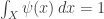
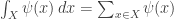
In general, this ‘evaluation at 1’ business is just a way of computing the sum of the coefficients of a power series:
Indeed, is the same as what I was calling
in my blog article: in this situation the ‘integral’ of means the sum of
  over all the possibilities
  .
.
So, in very terse notation which I haven’t quite defined yet but perhaps you can understand anyway, the th moment of the number of things can be written as
and this will come in handy.
To me all these tricks seem like mutant versions of familiar tricks in the quantum theory of the harmonic oscillator. To you they may seem like oddly worded restatements of familiar probability theory tricks!
Nico wrote:
It’s a ‘formal variable’, or ‘indeterminate’:
is a time-dependent formal power series.
You can think of as a real number if that helps, but that’s not quite right. The idea of a formal power series is that we don’t care if it converges; it’s just an abstract expression of the form
where the coefficients are (in this article) real numbers. So, for example,
is a perfectly acceptable formal power series even though it doesn’t converge when we try to set to some real number (other than
  ).
).
If you haven’t seen formal power series, they may seem strange, but they’re a very common and useful trick. You can think of a formal power series
as nothing but a cute way of packaging the infinite sequence . Any sequence gives a formal power series, called its generating function. Herbert Wilf wrote:
But generating functions are extremely useful, since operations like addition, multiplication, and differentiation of formal power series are efficient ways to manipulate sequences.
In an earlier comment, Tim van Beek pointed out Wilf’s book, which is free online:
• Herbert Wilf, Generatingfunctionology.
It’s a great book!
Maybe, but not necessarily. Note that
isn’t a function of . I’s just a formal power series in the variable
  which is a function of time,
  . It’s often handy to pretend that formal power series are functions, and if I were in that mood I’d write
But I preferred to honestly admit that is a formal-power-series-valued function of time, and write
For each time ,
,  is a formal power series in the formal variable
  .
.
Actually I agonized over these issues quite a bit, but I never considered writing . I was agonizing over whether to write
  or simply
  . I like short notations, and physicists (and some other people) often don’t explicitly write the variables that a function depends on. But I decided to write
  because some of my remarks concerned a time-dependent formal power series while other more general remarks, like the definition of creation operator:
apply equally well to time-independent and time-dependent ones—so there I used .
.
Sorry to be more dense than usual. Can’t the probabilities of the quantum models simply obey the same equations as the probabilistic model? Then the difference is that the quantum phases are important, and have interesting equations, while the probabilistic phases are boring.
John F wrote:
That seems tough. In a probabilistic model time evolution is linear in the probabilities. In a quantum model time evolution is linear in the amplitudes, and we square the absolute value of an amplitude to get a probability.
So, the challenge is to reconcile our requirement that time evolution be linear in both probabilities and amplitudes with the further requirement that probabilities depend nonlinearly on amplitudes!
More mathematically, what I’m saying is this. In a quantum model of the sort I’m talking about, time evolution of amplitudes is described by linear maps
In a probabilistic model, time evolution of probability distributions is described by linear maps
Taking the square of the absolute values gives a map from to
to  which sends amplitudes to probabilities. Let’s call it
  :
:
However, it’s hard to achieve
except for some very special cases. The only case I know is when both and
and  come from a 1-parameter family of measure-preserving maps
from our measure space to itself. It works like this:
These maps describe a deterministic time evolution of states in
  . The probability functions and wavefunctions just get dragged along by this deterministic time evolution. So, I know how to reconcile probabilistic and quantum models in the way you seem to be wanting… but only in the rather dull case where the dynamics is really deterministic!
This trick, with taken to be a classical ‘phase space’, can be used to make classical mechanics look superficially like quantum mechanics. It’s called ‘Koopmanism’ and it’s used in ergodic theory.
Hidden variables? I know, I know …
[…] Last time I told you what happens when we stand in a river and catch fish as they randomly swim past. Let me remind you of how that works. But today let’s use rabbits. […]
I think you forgot the keyword “latex” in $a^\dagger$ in the text 3 formulas before the end of the article.
Thanks – fixed! By the way, I answered the puzzle in Part 4. I hope the answer makes sense. If not, please ask a question!
[…] We need to recall the analogy we began sketching in Part 5, and push it a bit further. The idea is that stochastic mechanics differs from quantum mechanics in two ways […]
Sir,
Sorry if these questions are too elementary:
1. What is that way to make any set X into a measure space? Also, why do you say that integrals are more general than sums?
2. What is the meaning of conjugate linear?
3. Is there any difference between ‘maps’ and ‘functions’?
4. How do we know that is a vector space?
 – the first two terms are finite according to the definition of $L^2$, but how are we sure that the inner product will always be finite? Is there some other way to prove this?
–
5. The net-fish process in the beginning- The corresponding rate equation will be d(Nfish)/dt=r as the only species is fish and that does not appear as an input, so it’s power will be 0- Right?
Arjun wrote:
Use counting measure.
An integral with respect to counting measure is a sum. It sounds like you want to learn a bit about measure theory and Lebesgue integration, which is the theory of integration on general measure spaces.
Like most math terms, this is defined in Wikipedia. When I want to learn the meaning of a math term, I type it into Google, and usually a Wikipedia article shows up near the very top of the choices.
It depends on context. A ‘map’ is a function preserving whatever structure is on hand. For example if we talked about a map between topological spaces, we’d mean a continuous function. If we talked about a map between manifolds, we’d mean a smooth function. But a map between sets means a function.
(To add to the confusion, in the French tradition ‘function’ means a function taking values in the real or complex numbers, while a
general function is called a ‘map’.)
The Cauchy–Schwarz inequality holds for and it implies the triangle inequality, which proves
  is a vector space.
Right. Earlier you were asking about transitions with no inputs. I pointed you to this example.
1. Why should the Us be linear operators?
2. ” It seems easier to deal with this in the special case when integrals over X reduce to sums. So let’s suppose that happens… and let’s start by seeing what the first condition says in this case.
In this case, L^1(X) has a basis of ‘Kronecker delta functions’…”
– Can you help me understand this better?
3. I did not understand the paragraphs before the moral paragraph:
“…The idea behind my term is that any infintesimal stochastic operator should be the infinitesimal generator of a stochastic process.
In other words, when we get the details straightened out, any 1-parameter family of stochastic operators…
…Someone must have worked it out.”
4. The whole paragraph on Infinitesimal stochastic versus self-adjoint operators is not very clear to me, though I have read it 6-7 times.
I’ll only talk about the case where is stochastic, because I don’t want to explain why quantum mechanics is linear. I’ll just talk about why probability theory is linear.
Suppose we’re playing a game like this. If you give me $1, I’ll give you $1 with probability 90%, and nothing with probability 10%. If you give me nothing, I will give you nothing with probability 90%, and $1 with probability 10%.
Suppose you give me $1 with probability and nothing with probability
  After you play this game, you will have $1 with probability
  and nothing with probability
Calculate the vector as a function of
  In other words, write
  and tell me what the function
  is.
is.
If you do this example, it will help you see why we want to be linear.
You have to ask me a specific question for me to help you understand something better.
Again, that’s not a question. It’s a statement.
I hope you get the basic idea: if we have a bunch of linear operators we call
  the infinitesimal generator of those operators. I want to know which operators
  make
make  be stochastic for all
  I say a lot more about this in Part 12.
Again, that’s not a question. Have you tried doing some computations with examples? There are some things we can only learn by doing. We’ll do lots of calculations with infinitesimal stochastic operators in this course; for self-adjoint operators you’d do lots of calculations in a course on quantum mechanics.
Sorry for being so vague in my questions/statements- would not happen again. The paragraph is much clearer now.
Why do you say that ‘It is enough to assume t is very small’, when discussing about the nature of H for exp(tH) to be stochastic for all ? After that, how can we assume that the infinitesimal stochastic operator H will work to make exp(tH) stochastic for all times? Has it got something to do with these conditions on U:
 .
.
U(t)U(s) = U(t+s) and