
It’s time to continue this information geometry series, because I’ve promised to give the following talk at a conference on the mathematics of biodiversity in early July… and I still need to do some of the research! 
Diversity, information geometry and learning
As is well known, some measures of biodiversity are formally identical to measures of information developed by Shannon and others. Furthermore, Marc Harper has shown that the replicator equation in evolutionary game theory is formally identical to a process of Bayesian inference, which is studied in the field of machine learning using ideas from information geometry. Thus, in this simple model, a population of organisms can be thought of as a ‘hypothesis’ about how to survive, and natural selection acts to update this hypothesis according to Bayes’ rule. The question thus arises to what extent natural changes in biodiversity can be usefully seen as analogous to a form of learning. However, some of the same mathematical structures arise in the study of chemical reaction networks, where the increase of entropy, or more precisely decrease of free energy, is not usually considered a form of ‘learning’. We report on some preliminary work on these issues.
So, let’s dive in! To some extent I’ll be explaining these two papers:
• Marc Harper, Information geometry and evolutionary game theory.
• Marc Harper, The replicator equation as an inference dynamic.
However, I hope to bring in some more ideas from physics, the study of biodiversity, and the theory of stochastic Petri nets, also known as chemical reaction networks. So, this series may start to overlap with my network theory posts. We’ll see. We won’t get far today: for now, I just want to review and expand on what we did last time.
The replicator equation
The replicator equation is a simplified model of how populations change. Suppose we have 
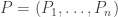
Let 


So, the population 


Of course this model is absurdly general, while still leaving out lots of important effects, like the spatial variation of populations, or the ability for the population of some species to start at zero and become nonzero—which happens thanks to mutation. Nonetheless this model is worth taking a good look at.
Using the magic of vectors we can write
and

This lets us write the replicator equation a wee bit more tersely as

where on the right I’m multiplying vectors componentwise, the way your teachers tried to brainwash you into never doing:

In other words, I’m thinking of 


Why would we want to do that? Well, we might be studying lizards with different length tails, and we might find it convenient to think of the set of possible tail lengths as the half-line 
Or, just to get started, we might want to study the pathetically simple case where 


If we’re physicists, we might write 


This looks a lot like Schrödinger’s equation, but since there’s no factor of 
For an explanation of Schrödinger’s equation and the master equation, try Part 12 of the network theory series. In that post I didn’t include a minus sign in front of the 
The replicator equation in terms of probabilities
Luckily, that’s exactly what people usually do! Instead of talking about the population 

Don’t you love it when notations work out well? Our big Population
How do these probabilities
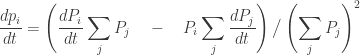
Using our earlier version of the replicator equation, this gives:
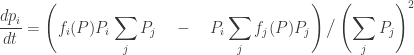
Using the definition of 
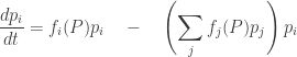
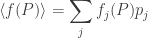
The stuff in parentheses actually has a nice meaning: it’s just the mean fitness. In other words, it’s the average, or expected, fitness of an organism chosen at random from the whole population. Let’s write it like this:
So, we get the replicator equation in its classic form:

This has a nice meaning: for the fraction of organisms of the
Entropy
Now for something a bit new. Once we’ve gotten a probability distribution into the game, its entropy is sure to follow:
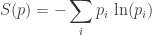
This says how ‘smeared-out’ the overall population is among the various different species. Alternatively, it says how much information it takes, on average, to say which species a randomly chosen organism belongs to. For example, if there are 


In biology, entropy is one of many ways people measure biodiversity. For a quick intro to some of the issues involved, try:
• Tom Leinster, Measuring biodiversity, Azimuth, 7 November 2011.
• Lou Jost, Entropy and diversity, Oikos 113 (2006), 363–375.
But we don’t need to understand this stuff to see how entropy is connected to the replicator equation. Marc Harper’s paper explains this in detail:
• Marc Harper, The replicator equation as an inference dynamic.
and I hope to go through quite a bit of it here. But not today! Today I just want to look at a pathetically simple, yet still interesting, example.
Exponential growth
Suppose the fitness of each species is independent of the populations of all the species. In other words, suppose each fitness 


so it’s easy to solve:

You don’t need a detailed calculation to see what’s going to happen to the probabilities
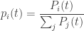
The most fit species present will eventually take over! If one species, say the 

and
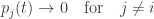
Thus the probability distribution 
With a bit more thought you can see that even if more than one species shares the maximum possible fitness, the entropy will eventually decrease, though not approach zero.
In other words, the biodiversity will eventually drop as all but the most fit species are overwhelmed. Of course, this is only true in our simple idealization. In reality, biodiversity behaves in more complex ways—in part because species interact, and in part because mutation tends to smear out the probability distribution 
In still other words, the population will absorb information from its environment. This should make intuitive sense: the process of natural selection resembles ‘learning’. As fitter organisms become more common and less fit ones die out, the environment puts its stamp on the probability distribution 
While intuitively clear, this last claim also follows more rigorously from thinking of entropy as negative information. Admittedly, it’s always easy to get confused by minus signs when relating entropy and information. A while back I said the entropy
was the average information required to say which species a randomly chosen organism belongs to. If this entropy is going down, isn’t the population losing information?
No, this is a classic sign error. It’s like the concept of ‘work’ in physics. We can talk about the work some system does on its environment, or the work done by the environment on the system, and these are almost the same… except one is minus the other!
When you are very ignorant about some system—say, some rolled dice—your estimated probabilities 
So, the entropy
It works the same way with our population of replicators—at least in the special case where the fitness of each species is independent of its population. The probability distribution
Next time
Of course, to make closer contact to reality, we need to go beyond the special case where the fitness of each species is a constant! Marc Harper does this, and I want to talk about his work someday, but first I have a few more remarks to make about the pathetically simple special case I’ve been focusing on. I’ll save these for next time, since I’ve probably strained your patience already.


“This should make intuitive sense: the process of natural selection resembles ‘learning’.”
Nature is one tough teacher.
Yes: only students who pass every test get to live.
Amazing how fast even microbes ‘learn’ with such a strict teacher.
The sum in the denominator of should probably be indexed by j.
Okay, I’ll do something like that.
Replicators with dispersion in rates and adaptation times could probably explain the huge dynamic range in relative abundance distributions. This was touched on in Part 8.
I’ll have to think about that!
I think the use of phrases like “absorb information from the environment” are a little too passive. I’d say a more informative analogy is that processes “acquire information from the environment”, with the process of acquisition being limited to asking questions of the form “I think x is a good answer, am I right?” (i.e., not just yes-no questions but yes-no questions about very specific things). Of course, the diff eqn framework you’re looking at doesn’t use the notion of the fitness of offspring being some function (either stochastic or some other type) of the parents fitness, so there’s no analogue of this effect in what you’re directly looking at.
But in looking for links between information theory and biology, particularly biodiversity, I’d be inclined to look at how information theory looks at the “question strategy” issues. (E.g., if you really want to maximise your probability of getting some right answer, you’re best served by testing “answers” at widely spaced parts of the configuration space, but biological evolution seems to churn out individuals who are only slightly different from their parents. Why is that? One quick possibility is that “evolutionary inference” thinks the parents are already quite close to the answer, so small modifications are called for. Or maybe it’s one or multiple other reasons…)
David wrote:
Evolutionary biologists are trained to avoid ‘teleological’ or ‘purposive’ accounts:
This is important for avoiding some mistakes. But I think it’ll be very interesting for evolutionary biology to collide with machine learning, where people with goals are designing systems in order to achieve those goals. Deen Abiola’s comments below show what I mean.
Here you’re talking about what evolutionary inference “thinks”, which would give you a rap on the knuckles in those biology courses.
More seriously, but relatedly, biologists are really interested in to what extent we can think of evolution itself as having been optimized for something… instead of just being a fixed method whereby other things get optimized. The buzzword for this puzzle is the evolution of evolvability:
If you allow me to display my ignorance here: doesn’t this depend on what you assume as possible for ? (for example, the constant
  )
)
Suppose we take two species and
and  who have some symbiotic relationship, but have to share a finite area. E.g. suppose that (
 is a positive coefficient):
and similar for , but with
  and
and  exchanged.
Then for large
 and
and  will both go to 1/2. Also in this case I would say that the replicators gathered information about their environment (even though this example may not be very realistic) however it appears to me that the entropy becomes maximal. Am I doing something wrong?
Frederik wrote:
Yes! My remarks in the section “Exponential growth” only apply to the pathetically simple special case where is actually independent of
  , so the population of each species grows or declines exponentially. This is a very boring case, and it would be almost silly to even mention it except that for short times, we can approximate the solution of any equation
by a solution of the linear equation
This is my ultimate reason for introducing the pathetically simple special case. However, you’ll note that in this section, I only analyze the behavior of this case as . So, the lessons here won’t apply to more general cases—at least, not without tons of qualifications. Next time I’ll look at the short-time behavior of the same pathetically simple special case, and get some more lessons.
I should have made this more clear. I’m not explaining things very well since I’m learning it and/or making it up as I go.
Your example is a nice one, since it illustrates the importance of inter-species interactions, which are completely absent in the pathetically simple special case I discussed. I’ll talk more about those later!
There’s a lot of interesting stuff to say about how information flows in situations where species are competing or cooperating with each other, but it’s more complicated than “so, the entropy drops”. Very often it rises.
For now, try this:
• Marc Harper, The replicator equation as an inference dynamic.
Last time I began explaining the tight relation between three concepts: entropy, information and biodiversity […]
Hi John!
I’m happy to see that you are still interested in the topics. I want to recognize some other researchers that have had similar ideas (and that I based some of my work on). In particular, Cosma Shalizi independently discovered the analogy between the discrete replicator dynamic and Bayesian inference; I.M. Bomze was the first (as far as I can tell) to use relative entropy / cross entropy to analyze the replicator dynamic and proved many important results; and Shun-ichi Amari and his many collaborators wrote briefly about the connection between information geometry and the replicator equation circa 1995 and in subsequent works.
Unfortunately I found out about much of these researchers’ work after I had finished my graduate thesis — some of it would have been much easier to figure out! In any case, there’s credit where credit is due!
Over on G+, Deen Abiola wrote:
John Baez wrote:
Deen Abiola wrote:
Deen Abiola wrote:
Marc Harper wrote:
Deen Abiola wrote:
In Part 9, I told you about the ‘replicator equation’, which says how these fractions change with time […]
This would be a version of the replicator equation, which I explained recently in Information Geometry (Part 9). […]
I have been intrigued by the similarity of the definition of entropy to the formula for the n’th prime number;
p(n) = n*ln(n) + …
Is this similarity only accidental or does it have a meaning?
This is my talk for the workshop Biological Complexity: Can It Be Quantified?
• Biology as information dynamics.