Last time I gave a sketchy overview of evolutionary game theory. Now let’s get serious.
I’ll start by explaining ‘Nash equilibria’ for 2-person games. These are situations where neither player can profit by changing what they’re doing. Then I’ll introduce ‘mixed strategies’, where the players can choose among several strategies with different probabilities. Then I’ll introduce evolutionary game theory, where we think of each strategy as a species, and its probability as the fraction of organisms that belong to that species.
Back in Part 9, I told you about the ‘replicator equation’, which says how these fractions change with time thanks to natural selection. Now we’ll see how this leads to the idea of an ‘evolutionarily stable strategy’. And finally, we’ll see that when evolution takes us toward such a stable strategy, the amount of information the organisms have ‘left to learn’ keeps decreasing!
Nash equilibria
We can describe a certain kind of two-person game using a payoff matrix, which is an 


Note that in this kind of game, there’s no significant difference between the ‘first player’ and the ‘second player’: either player wins an amount 

We say a strategy

for all 
For example, suppose our matrix is

Then we’ve got the Prisoner’s Dilemma exactly as described last time! Here strategy 1 is cooperate and strategy 2 is defect. If a player cooperates and so does his opponent, he wins

meaning he gets one month in jail. We include a minus sign because ‘winning a month in jail’ is not a good thing. If the player cooperates but his opponent defects, he gets a whole year in jail:

If he defects but his opponent cooperates, he doesn’t go to jail at all:

And if they both defect, they both get three months in jail:

You can see that defecting is a Nash equilibrium, since

So, oddly, if our prisoners know game theory and believe Nash equilibria are best, they’ll both be worse off than if they cooperate and don’t betray each other.


Nash equilibria for mixed strategies
So far we’ve been assuming that with 100% certainty, each player chooses one strategy 
Now let’s throw some probability theory into the stew! Let’s allow the players to pick different pure strategies with different probabilities. So, we define a mixed strategy to be a probability distribution on the set of pure strategies. In other words, it’s a list of 

that sum to one:

Say I choose the mixed strategy 


so the expected value of my winnings is

or using vector notation

where the dot is the usual dot product on

We can easily adapt the concept of Nash equilibrium to mixed strategies. A mixed strategy 

This means that if both you and I are playing the mixed strategy 

If this were a course on game theory, I would now do some examples. But it’s not, so I’ll just send you to page 6 of Sandholm’s paper: he looks at some famous games like ‘hawks and doves’ and ‘rock paper scissors’.
Evolutionarily stable strategies
We’re finally ready to discuss evolutionarily stable strategies. To do this, let’s reinterpret the ‘pure strategies’ 
Similarly, we’ll reinterpret the ‘mixed strategy’ 

We’ll reinterpret the payoff matrix 

where the fitness function 
But in evolutionary game theory it’s common to start by looking at a simple special case where

where

is the fraction of replicators who belong to the
What does this mean? The idea is that we have a well-mixed population of game players—or replicators. Each one has its own pure strategy—or species. Each one randomly roams around and ‘plays games’ with each other replicator it meets. It gets to reproduce at a rate proportional to its expected winnings.
This is unrealistic in all sorts of ways, but it’s mathematically cute, and it’s been studied a lot, so it’s good to know about. Today I’ll explain evolutionarily stable strategies only in this special case. Later I’ll go back to the general case.
Suppose that we select a sample of replicators from the overall population. What is the mean fitness of the replicators in this sample? For this, we need to know the probability that a replicator from this sample belongs to the 

This is just a weighted average of the fitnesses in our earlier formula. But using the magic of vectors, we can write this sum as

We already saw this type of expression in the last section! It’s my expected winnings if I play the mixed strategy
John Maynard Smith defined 
In simple terms: a small ‘invading’ population will do worse than the population as a whole.
Mathematically, this means:

for all mixed strategies 

is the population we get by replacing an 
Puzzle: Show that

and also, for all 

The first condition says that
Again, I should do some examples… but instead I’ll refer you to page 9 of Sandholm’s paper, and also these course notes:
• Samuel Alizon and Daniel Cownden, Evolutionary games and evolutionarily stable strategies.
• Samuel Alizon and Daniel Cownden, Replicator dynamics.
The decrease of relative information
Now comes the punchline… but with a slight surprise twist at the end. Last time we let
be a population that evolves with time according to the replicator equation, and we let
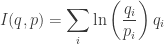
obeys

where 

for all 
We can adapt this to the special case we’re looking at now. Remember, right now we’re assuming
so

Thus, the relative information will never increase if

or in other words,

Now, this looks very similar to the conditions for an evolutionary stable strategy as stated in the Puzzle above. But it’s not the same! That’s the surprise twist.
Remember, the Puzzle says that

and also

Note that condition (1), the one we want, is neither condition (2) nor condition (3)! This drove me crazy for almost a day.

I kept thinking I’d made a mistake, like mixing up
But the solution turned out to be this. After Maynard Smith came up with his definition of ‘evolutionarily stable state’, another guy came up with a different definition:
• Bernhard Thomas, On evolutionarily stable sets, J. Math. Biology 22 (1985), 105–115.
For him, an evolutionarily stable strategy obeys
and also
Condition (1) is stronger than condition (3), so he renamed Maynard Smith’s evolutionarily stable strategies weakly evolutionarily stable strategies. And condition (1) guarantees that the relative information 
Except for one thing: why should we switch from Maynard Smith’s perfectly sensible concept of evolutionarily stable state to this new stronger one? I don’t really know, except that
• it’s not much stronger
and
• it lets us prove the theorem we want!
So, it’s a small mystery for me to mull over. If you have any good ideas, let me know.


There are some typos in the subscripts when you’re discussing the payoff matrix for the prisoner’s dilemma: is used three times when you mean
  and
and  for the last two equations.
Thoughtless cut-and-paste on my part… rushing to finish this post. Thanks, I’ll fix those typos!
I think I can shed some light on the distinctions between the conditions (1) and (3). Many authors use the implication of condition (3) (i.e. strict inequality in condition (1)) as the definition of ESS. Indeed, one can show that the strict version of (1) holds in some neighborhood of q if and only if q is an ESS (for a proof, see theorem 6.4.1 in Hofbauer and Sigmond’s “Evolutionary Games and Population Dynamics”). So the question is why we want the inequality to be strict intuitively. I’ll give a few examples why strictness matters.
The derivative of I being zero does not imply that the dynamic is stationary. Sometimes I is a constant of motion (e.g. for the rock-scissors-paper game), which has concentric orbits about the center of the simplex in dimension three. These orbits are not attractive (there is no limit cycle), so while the population is stuck on a particular cycle based on the initial point and is in some sense stable, it is not stable in the intuitive sense of evolutionary/selective stability. It makes sense that the relative entropy (with q being the center of all the cycles, which is a stable point, but not asymptotically so) is constant on these cycles — there is no information gain for otherwise the dynamic would not cycle.
Another situation is that one can have an evolutionarily stable set for a particular game matrix A, for instance, a connected line of stable points such that the set is locally asymptotically stable, but that there is no motion along the line, so that no point in the line is distinguished as locally asymptotically stable. In three dimensions it would look something like this (http://ars.els-cdn.com/content/image/1-s2.0-S0370157307001810-gr4.jpg) if all those points were connected in a line across the ternary plot. The matrix given by equation (7.20) in Hofbauer and Sigmond produces such a set of equilibria.
In this case, we don’t have have evolutionary stability in the sense of Maynard Smith because points q on the line are not resistant to invasion. In other words, condition (3) would not be satisfied because with the influx of a particular distribution of mutants (shifting along the line of equilibria from q to p), the population would not tend back to the distribution before the influx, and so the point q is not selectively stable, and this holds for every point on the line. If an evolutionarily stable set is a single point, then it would typically be an evolutionarily stable state.
Finally, some more mathematical reasons: there are different conclusions from the Lyapunov stability theorem if the derivative of the relative entropy I is always negative versus just non-positive, namely that the equilibrium is locally asymptotically stable rather than just stable. Also, Ross Cresmann showed that evolutionary stability is equivalent to the dynamical system notion of strong stability, which many find to be intuitively satistifying.
I’m in favor of John Maynard Smith’s definition. It comes from basic biological considerations. In his definition, a strategy is evolutionarily stable iff it is impossible for a small group of invaders with a different strategy to displace a resident population that is already using this strategy. In short, “evolutionarily stable” means “robust to small groups of invaders”. Of course, there is a biological reason for thinking about small groups of invaders: new types typically arise in small numbers, either through mutation or migration.
In the replicator dynamics, Maynard Smith’s ESS definition implies local asymptotic stability.
Bernhard Thomas’s definition, on the other hand, says that strategy q beats or ties any other strategy distribution it is competing with, whether rare or common. It is equivalent to saying that q is an ESS if for any other distribution p and any proportion x of strategy p,
q.[(1-x)q+xp] >= p.[(1-x)q+xp]
So, no matter what proportions q and p are blended in, q wins or ties.
To me, this doesn’t fit the name “evolutionarily stable”. I think it should instead be something like “evolutionarily dominant”. In this view “evolutionarily stable” means you’re safe against small group of invaders, but another strategy could still displace you if it arrives in sufficiently large numbers. “Evolutionarily dominant” means that nothing can beat you. (This distinction is relevant in many biological situations.)
Also, it’s not true that Thomas’s definition is strictly stronger than Maynard Smiths, at least not in the way you’ve written them. This is because the inequality in (3) is strict while the inequality in (1) is not.
If we strengthen Thomas’s definition by making the inequality in (1) strict for all p != q, then this strengthened version of (1) implies that q is a global attractor for the replicator dynamics. So in some sense, Maynard Smith’s definition is about local stability, and Thomas’s definition is about global stability.
After having thought about this some more, I agree even more that Maynard Smith’s definition matches our intuition of ‘evolutionary stability’… but Thomas’ definition is important too, at least because we need it to prove this version of the 2nd law of thermodynamics. I like your idea of naming this concept ‘evolutionary dominance’. In my talk in Barcelona I used the term ‘evolutionary optimum’, but ‘evolutionary dominance’ captures the idea better. I’ll use that from now on!
I should pay more attention to versus
  . In Marc Harper’s theorem I was content to have a non-strict inequality, so I used a non-strict inequality in the definition, but a strict inequality in the definition should give a strict inequality in the theorem, as long as
  . Thanks!
If makes this true for all
  we say
  is an evolutionarily stable state. For some reasons why, see Part 13.
This is my talk for the workshop Biological Complexity: Can It Be Quantified?
• Biology as information dynamics.