Sometimes patterns can lead you astray. For example, it’s known that

is a good approximation to 


and

But in 1914, Littlewood heroically showed that in fact, 
This raised the question: when does 


Later, in 1955, Skewes showed without the Riemann hypothesis that

By now this bound has been improved enormously. We now know the two functions cross somewhere near 
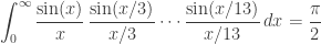
All this math is quite deep. Here is something less deep, but still fun.
You can show that


and so on.
It’s a nice pattern. But this pattern doesn’t go on forever! It lasts a very, very long time… but not forever.
More precisely, the identity
holds when

but not for all 

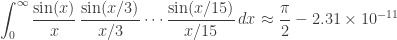
The explanation
The integrals here are a variant of the Borwein integrals:


where the pattern continues until
but then fails:
I never understood this until I read Greg Egan’s explanation, based on the work of Hanspeter Schmid. It’s all about convolution, and Fourier transforms:
Suppose we have a rectangular pulse, centred on the origin, with a height of 1/2 and a half-width of 1.
Now, suppose we keep taking moving averages of this function, again and again, with the average computed in a window of half-width 1/3, then 1/5, then 1/7, 1/9, and so on.
There are a couple of features of the original pulse that will persist completely unchanged for the first few stages of this process, but then they will be abruptly lost at some point.
The first feature is that F(0) = 1/2. In the original pulse, the point (0,1/2) lies on a plateau, a perfectly constant segment with a half-width of 1. The process of repeatedly taking the moving average will nibble away at this plateau, shrinking its half-width by the half-width of the averaging window. So, once the sum of the windows’ half-widths exceeds 1, at 1/3+1/5+1/7+…+1/15, F(0) will suddenly fall below 1/2, but up until that step it will remain untouched.
In the animation below, the plateau where F(x)=1/2 is marked in red.

The second feature is that F(–1)=F(1)=1/4. In the original pulse, we have a step at –1 and 1, but if we define F here as the average of the left-hand and right-hand limits we get 1/4, and once we apply the first moving average we simply have 1/4 as the function’s value.
In this case, F(–1)=F(1)=1/4 will continue to hold so long as the points (–1,1/4) and (1,1/4) are surrounded by regions where the function has a suitable symmetry: it is equal to an odd function, offset and translated from the origin to these centres. So long as that’s true for a region wider than the averaging window being applied, the average at the centre will be unchanged.
The initial half-width of each of these symmetrical slopes is 2 (stretching from the opposite end of the plateau and an equal distance away along the x-axis), and as with the plateau, this is nibbled away each time we take another moving average. And in this case, the feature persists until 1/3+1/5+1/7+…+1/113, which is when the sum first exceeds 2.
In the animation, the yellow arrows mark the extent of the symmetrical slopes.
OK, none of this is difficult to understand, but why should we care?
Because this is how Hanspeter Schmid explained the infamous Borwein integrals:
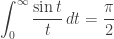
∫sin(t)/t dt = π/2
∫sin(t/3)/(t/3) × sin(t)/t dt = π/2
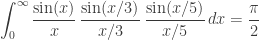
∫sin(t/5)/(t/5) × sin(t/3)/(t/3) × sin(t)/t dt = π/2…
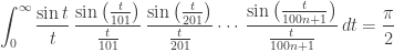
∫sin(t/13)/(t/13) × … × sin(t/3)/(t/3) × sin(t)/t dt = π/2
But then the pattern is broken:
∫sin(t/15)/(t/15) × … × sin(t/3)/(t/3) × sin(t)/t dt < π/2
Here these integrals are from t=0 to t=∞. And Schmid came up with an even more persistent pattern of his own:
∫2 cos(t) sin(t)/t dt = π/2
∫2 cos(t) sin(t/3)/(t/3) × sin(t)/t dt = π/2
∫2 cos(t) sin(t/5)/(t/5) × sin(t/3)/(t/3) × sin(t)/t dt = π/2
…
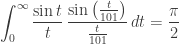
∫2 cos(t) sin(t/111)/(t/111) × … × sin(t/3)/(t/3) × sin(t)/t dt = π/2But:
∫2 cos(t) sin(t/113)/(t/113) × … × sin(t/3)/(t/3) × sin(t)/t dt < π/2
The first set of integrals, due to Borwein, correspond to taking the Fourier transforms of our sequence of ever-smoother pulses and then evaluating F(0). The Fourier transform of the sinc function:
sinc(w t) = sin(w t)/(w t)
is proportional to a rectangular pulse of half-width w, and the Fourier transform of a product of sinc functions is the convolution of their transforms, which in the case of a rectangular pulse just amounts to taking a moving average.
Schmid’s integrals come from adding a clever twist: the extra factor of 2 cos(t) shifts the integral from the zero-frequency Fourier component to the sum of its components at angular frequencies –1 and 1, and hence the result depends on F(–1)+F(1)=1/2, which as we have seen persists for much longer than F(0)=1/2.
• Hanspeter Schmid, Two curious integrals and a graphic proof, Elem. Math. 69 (2014) 11–17.
I asked Greg if we could generalize these results to give even longer sequences of identities that eventually fail, and he showed me how: you can just take the Borwein integrals and replace the numbers 1, 1/3, 1/5, 1/7, … by some sequence of positive numbers

The integral
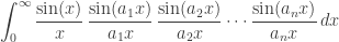
will then equal 

• Wikipedia, Borwein integral: general formula.
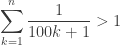
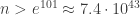
As an example, I chose the integral
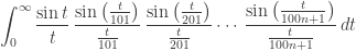
which equals
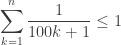
Thus, the identity holds if

However,
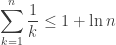
so the identity holds if
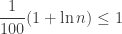
or

or
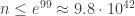
On the other hand, the identity fails if
so it fails if

However,

so the identity fails if

or

or
With a little work one could sharpen these estimates considerably, though it would take more work to find the exact value of 
first fails.


There’s a typo in the definition of li(x)
Whoops! I’ll fix it, thanks.
I believe the first for which the pattern fails is:
15,341,178,777,673,149,429,167,740,440,969,249,338,310,889
The sum can be rewritten in terms of digamma functions:
which Mathematica can calculate with a Taylor series (or something similar), so it’s possible to evaluate it to sufficient precision to be sure that the value is greater than 1 for this , and less than 1 for
  .
.
And the Schmid integrals, with their extra factor of , will stick to the pattern until the sum first exceeds 2, at
  equal to:
412,388,856,479,291,008,968,946,990,055,780,778,304,566,005,151,152,521,580,673,941,188,473,456,899,173,626,864,612
Greg wrote:
That’s great! I should have read your comment before I tweeted about this today, so I could include the exact number. But I composed the tweet yesterday after merely working out an estimate.
I didn’t know that the digamma function
obeys
So, I didn’t know a good strategy to compute the exact number.
The explanation by Greg and Schmid is really insightful. Rademacher functions are step functions (the Fourier transform of the sinc function gets you back to the square wave) and the integral of the product of them over (0,1) is zero :
 for any n
regarding patterns, I see this in the news:
“Famed mathematician claims proof of 160-year-old Riemann hypothesis:
https://www.newscientist.com/article/2180406-famed-mathematician-claims-proof-of-160-year-old-riemann-hypothesis/
Yes, and you can see my response on Twitter, but I don’t really want to talk about that here.
More relevant is the question of whether numerical evidence for the Riemann hypothesis is really convincing!
In 2000, Gourdon and Demichel showed that the first 10,000,000,000,000 nontrivial zeros of the Riemann zeta function lie on the line Re(z) = 1/2, just as the Riemann hypothesis claims. They also checked two billion much larger zeros.
Normally this would seem pretty convincing. But some argue otherwise! According to Wikipedia:
Emphasis mine.
People forget how large finite numbers can be. There are finite numbers so large that our civilization will never be able to write them down. And I am pretty sure that by undecidability of arithmetic there is no bound on the sizes of counterexamples to propositions, which means that for any finite n there is a proposition that fails for all m>=n. So there is the danger that we could run into a conjecture with one of those unreachable counterexamples.
Well, it makes it at least valid as a physical theory then. Except we don’t have explanation for it, or prime principles.
I think there is a typo in the condition on . It should be
  .
.
You’re right—or I should write the integral as
[…] A mathematical pattern that fails after about 10^43 examples 5 by fanf2 | 0 comments on Hacker News. […]
Well, considering series which is always less than 1,
is always equal to
That’s a nice idea!
I think this could help: https://doi.org/10.1088/1751-8121/aa6f32
iop.org paywall BS? Really?
https://arxiv.org/abs/1610.09702 please!
As things stand, I read your discussion of how you found the bounds on the range of where your example first fails as saying, for example,
(i.e., that the first statement, and the second notionally opposed statement, have to hold). I think that it would be clearer with commas (which would, perhaps unfortunately, have to be part of the displayed math):
to emphasise that the ‘but’ is helping you narrow down the range of to be considered, not directly imposing a further condition on
  .
.
Good point! I’m glad someone is reading this stuff in a careful and critical way.
Instead of making one little comma carry such a heavy burden, I think I’ll deploy that wonderful word “However”.
The Borweins have been at this stuff for a while – see their 2007 paper with Robert Baillie, “Surprising Sinc Sums and Integrals” which sets out the Fourier theoretic background to the compelling visual explanations give by Greg Egan and Hanspeter Schmid.
In Fourier theoretic terms you are transforming, via convolutions, a unitbox signal which gets you to a sinc wave in the transform space. Along the way you get the “localisation –nonlocalisation effect” ie if something is concentrated in interval of length L then in the transform space it cannot be located in an interval essentially less than 1/L – Heisenberg uncertainty if you like, but really just a property of Fourier transforms. It is still surprising that the pattern breaks down and Hanspeter Schmid really nails it by referring to the erosion on the plateau of the box function in the convolution process. He has come at it from a signal processing angle I think.
As an aside Jonathan Borwein died in 2016 while at Newcastle University, Australia. He was a Fellow of the Australian Academy of Sciences.
It’s just a cheap variation of what you discussed in the post, and works for a simpler version of the same reason.
Yes, that’s nice!
The link for the animation is broken; I think it has an extra closing parenthesis.
As an irrelevant analogy this reminds me of somone who is driving a car , and who has a series of drinks, each smaller than the previous one, Eventually they may go off the road and stop.
I felt lost until I reached this point: “I never understood this…”
Yes. I’m only human. But the next word was “until”.
One fun part of math is how a shocking, mysterious fact can suddenly become obvious when you look at it the right way.
But often, looking at it the right way requires preparation. Looking at the Borwein integrals in the right way requires some familiarity with how the Fourier transformation turns convolution into multiplication, and step functions into sinc functions. This is the sort of thing any good electrical engineer or physicist would know. I’m not sure all mathematicians get sufficient training in the nitty-gritty of such things, these days. Or maybe I’m just hanging out with too many would-be category theorists.
One of the best pieces of advice I could think to give the would-be category theorists is: keep learning all sorts of mathematics. Those other sorts of mathematics might need you some day!
More and more I see evidence of over-specialization, where people who seem very sophisticated in certain aspects of category theory are uncomfortable with basic topics first taught at the undergraduate level. (And one thing that impressed me about Russian mathematical culture, at least in those coming from the Soviet era, was the sheer breadth of their knowledge. It seemed to be a point not to over-specialize.)
I’m sometimes intimidated by young mathematicians who know (∞,1)-categories and the like better than I do… until I say something about other branches of math or physics and discover they are completely clueless about many basic facts. Then I’m reassured that my life hasn’t actually been wasted.
For example, I remember explaining to some mathematicians why the Moon rises a bit later each day. I can easily imagine not remembering whether it’s earlier or later. But this is something one can work out from first principles if one knows the Moon orbits the same way the Earth turns. Given that fact, a good mathematician should be able to figure out pretty quickly about much later the Moon rises each day. If they can’t do that, no amount of (∞,1)-categorical expertise will impress me.
I also remember stumping people with the question “if a solar eclipse happens when the Moon comes between the Sun and the Earth, why isn’t there one every month?”
A more significant challenge: “Since all rocks come from material that formed the Earth about 3 or 4 billion years ago, how can we use radioactive dating to measure the age of rocks and get different answers for different rocks?”
And: “If hot air rises, why is it colder on mountain tops?”
I usually don’t like to be put on the spot with those types of physics questions, the kind that ‘only’ require reasoning your way through them starting from first principles. Sort of like how I don’t like being put on the spot by logic puzzles. I may be happy to think about them in a leisurely moment by myself, but on the spot and in public they are likely to make me feel dumb — I’m not that quick on my feet for questions where I don’t have much practice. (All the same, I did enjoy your questions!)
I ball-parked the moon question just by assuming a 30-day revolution around the earth (from the observer’s eye) as opposed to a 24 hour rotation, and then dividing 24 by 30, multiply by 60, to get the number of minutes difference for each day. That’s 48 minutes. Add a little to that since the revolution is a little less than 30 days. That’s not an explanation of course, just a number.
Anyway, I hope the would-be category theorists don’t ignore or let themselves be turned off from analysis. Personally I often enjoy calculating, and I find a kind of charm in special functions (like sinc). These days I’m tutoring a 14-year-old budding mathematician who recently wanted to learn about the Gamma function, and I wound up learning all sorts of fun things. A mathematician should never get so sophisticated that such topics are pooh-poohed as beneath one’s dignity.
I don’t love being put on the spot by puzzles either. I used to really hate it, but I think I’ve relaxed because James Dolan taught me a lot of category theory by bombarding me with puzzles, and I got used to fumbling around out loud with him occasionally giving hints. Typical examples: “what’s a comonoid in the category of sets?” and “what’s a monoid in the category of monoids?” So now I tolerate it. If I don’t know, I don’t know.
I don’t judge people by their ability to solve puzzles quickly. But I do get judgemental when I meet mathematicians and physicists who seem not to have thought about many of the puzzles that naturally come up when you look at the world with a scientific eye—meaning, an eye that wants explanations of things. For example, everyone loves to say that “heat rises”, and yet a snow-capped mountain is practically a cliche. What does it mean about someone if they’ve never wondered about this? Do they just take the world at face value as an arbitrary collection of tendencies? “Shit happens”? I have trouble sympathizing with this outlook. Maybe I’m being unfair. Maybe they were slapped down a few many times when they asked questions as a child.
That’s fine!
Here’s how I’d explain it to someone, while sliding coins around on a table to illustrate everything. Imagine a penny orbiting a quarter, while the quarter turns in the same direction. The penny is the Moon and the quarter is the Earth. Say the penny goes around the quarter once every month, while the quarter turns around once a day. Since they’re turning the same way, a little guy standing on the Earth will see the Moon come into a view a bit later than if the Moon were just sitting there: he has to ‘catch up’ with the Moon. The amount of ‘catch-up’ each day is the amount the Moon has moved in one day. That’s about 1/30th of a day, since a month is about 30 days. Since there 24 hours in a day, the Moon should rise a bit less than an hour later each day.
(And then if you look at at a table of moonrises you see it’s more complicated than that… but it’s roughly right.)
My own guess is that many people may have wondered about various phenomena when they were young and curious, but that in many cases, when they are old enough to find real answers to those questions, that curiosity has largely dissipated and they no longer care that much. Scientists, at least those working at the highest levels, carry their youthful curiosity into their adult years.
I learned from MacPherson, in his interview for the Simons Foundation (here, segment 13), about a theory that Kolmogoroff had. In all mammalian species, the young are playful and curious and are trying to find out about their world; in the adult stage those characteristics fade as the mature animal needs to care for the young, work with the pack to get food, etc. — with a consequent need for a stable world without too many surprises. Kolmogoroff believed that mathematicians and scientists, those working at high creative levels, must have somehow had their personalities “frozen” somewhere in the playful stage. And so he and Alexandroff would play games, trying to guess at the spiritual ages of their colleagues — some age between 4 years and 18, or so. Gelfand also subscribed to this theory and would tell people his estimate of their true age; MacPherson, for example, he thought was about 8. MacPherson for his part also believes the theory (and thinks Gelfand guessed more or less right in his case), and goes on to say that with Jim Simons he usually feels like a kid brother, whereas he estimates Deligne to be spiritually around 6, and usually feels a kind of protective urge towards him.
Probably this is amusing only for those who sort of buy into the idea. I like the idea myself. But it’s more subtle than “the younger you are spiritually, the more curious and playful you are” — there are indefinable qualia at work that guide one’s feelings about this.
I agree that ‘childlike curiosity’ seems to be required for really novel discoveries: raw ambition may drive one to solve a hard open problem, but it probably won’t help you notice a little thread sticking out from the fabric of mathematics and start pulling on it.
The downside of the puer aeternus approach to mathematics is that the men who embrace it often rely on other people, usually women, to take care of them. Think for example of Perelman living with his mother—or Erdös living with his mother until she died, coach-surfing at his coauthors’ houses, and not even knowing how to make toast. I don’t think women can get away with this behavior: it seems to be a guy thing.
Right. I guess I’ll keep this relatively short: puer aeternus is a term used especially in Jungian psychology for a complex or syndrome which combines those elements that Kolmogoroff et al. intuited with more negative elements which could be summarized as a refusal to grow up or face the hard facts of life. (The seminal text by von Franzen is completely fascinating by the way; I highly recommend it.) I think those Russian fellows, besides just having fun, were pointing to something broader than just the puer ‘type’ identified by Jung and his followers. Although I easily believe that Erdos [with the double umlaut] was a puer in the Jungian sense (I am less familiar with Perelman’s story). You’re right that it’s mostly identified with males, although Jung et al. also referred to puellae aeternae.
I have never even understood the difference between the Fourier and Laplace transforms (though i have seen many explanations –they are sort of like the difference between the classical diffusion equation and the schrodinger equation—one has an i=sqrt(-1), the other doesn’t. you can write down lagrangians for both of them. You can rewrite both of them as path integrals–feynman did the quantum case, M Kac did the classical case (although maybe others did these as well–maybe landau and lifshitz)
i view fourier series and its results as variants of Taylor’s series (using complex numbers). .
One thing i’ve seen in statistical physics (Ising model, potts model, spin glasses) is use of sinh and cosh functions. Like category theory, these are not easy to intuitively understand for me.
one idea i’m working on is step functions. make everything discrete.
Ishi wrote:
What do you mean? Given your knowledge of path integrals and the like, it sounds like you’re showing off a very sophisticated high-level lack of understanding. There is always more to understand, and deliberately “not understanding” something is a great way to dig to deeper levels of understanding.
It took me a long time to understand why electrical engineers like Laplace transforms more than Fourier transforms for certain applications, but then I taught a basic course that explained how to solve linear constant-coefficient ODE using Laplace transforms, and it became clear to me—at least at a rather unsophisticated level.
First, the Laplace transform of a function will be a well-defined function as long as
  is piecewise continuous and grows slower than exponentially, which is true for all reasonable signals. This is not true of the Fourier transform; there one will often get a distribution under these conditions. Second, initial conditions for ODE are automatically taken into account in a nice way when one does a Laplace transform, since
Again, the Fourier transform doesn’t work like this.
Maybe we’re talking at cross-purposes, but I’d said that the Fourier transform of a step function involves the sinc function. That’s different from the sinh function.
I don’t think anyone gets an intuition for functions of different kinds without using them a lot.
I have actually gone to the trouble of seeing how Laplace “did the business” with the transforms named after him. His monumental probability treatise contains a large slab of the theory of generating functions and the solution of linear difference equations. When you hack through the ancient typesetting you will find the basic concept but you won’t find any tables of transforms! But you can see the motivation. I’ve done a line by line exposition of how Laplace actually proved the central limit theorem: https://www.gotohaggstrom.com/The%20central%20limit%20theorem%20-%20how%20Laplace%20actually%20proved%20it_17Oct2015.pdf
and I may get around to doing the same for his development of Laplace transforms. The modern proofs of the CLT rely upon Fourier theory because of the role of the characteristic function (FT of probability density function). Historically, the Laplace transform is rooted in Laplace’s development of probability theory. Laplace transforms are used in asymptotic estimates, a famous example of which is Renyi’s parking problem in which Renyi used Laplace transforms to give an estimate for the expected number of cars of unit length able to park in a street of length x as given by the recursion
so that is about as big as
when is large (the Laplace transform was needed to demonstrate that estimate).
There is an amusing Youtube video of MIT’s Arthur Mattuck confessing that for years he has never explained where the Laplace transform comes from so he breaks from tradition and actually explains its genesis!
Many students have lived in fog of ignorance as a result.
Isn’t one concise way to show the CLT is apply the Laplace transform? The CLT is essentially convolution of Gaussians, convolution is a multiplication of the Laplace transform, the Laplace transform of a Gaussian is a Gaussian. Therefore one can see how the composite Gaussian narrows with repeated convolutions, which is the idea behind the CLT.
It’s easy to see that convolving Gaussians gives Gaussians; the point of the central limit theorem is to show that if you convolve a bunch of _non_Gaussians the result approaches a Gaussian under certain conditions.
But yes, the fact that convolving Gaussians gives a Gaussian again is a big hint.
@Peter Haggstrom: “The modern proofs of the CLT rely upon Fourier theory”. That’s too categorical a statement to be true. I’d go along with “The standard modern textbook proof of the CLT relies on Fourier theory”, but I’d say the real reason for that is that (1) authors of (graduate-level) probability texts feel they need to develop the Fourier theory anyway, and (2) if you’ve already invested a lot of time developing the necessary Fourier theory, the proof of the vanilla CLT is pretty easy. But there are lots of other approaches, even in textbooks. See here for a sampler of methods, both old and new(er), that modern probabilists use every day.
Thanks John Baez for your detailed response.
Your explanation of Laplace vs fourier transform makes sense and i’ve seen them before —i even have a few papers saved on my computer to read again to get my mind right if that is even possible (highly unlikely).
i actually knew sinc is not sinh–i just noticed they had similar letters. only one i had heard of was sinh –and again if i see the formula for sinh i don’t intuitively understand it unless they draw a picture with a computer. Ising model also uses tanh.
(in my limited math experience, the only pictures i saw were of linear equations–a straight line—and a quadratic equation. They had almost no pictures of polynomial equations. Same with statistics–you can see a picture or graph of a gaussian distribution, maybe a power law, but very few multimodal distributions (which were and may still be my main interest.
i’ve climbed alot of mountains—maybe one can turn these into a gaussian distribution —average the himalayas, kansas, sierra nevada and saharan desert –i’ve been in all those places and almost died in every one from cold, heat, thirst, starvation and violence. But my experience shows that you need more detail. In detail the world is not a normal distribution. You go from flat kansas to ‘hilly ‘ rocky mountains cross parts of flat nevada and then go over sierra nevada. on average the world is lfat or normally distributed. in practice it isn’t.
Since i dont work with laplace and fourier transforms everyday I don’t have an intuitive understanding of them.
(i first came across fourier transforms in quantum mechanics , where they are sort of the standard recipe especially at undergrad level–uncertainty principal–i think there is a result from statistics called cramer-rao theorem (or something) that gives you something similar to heisenberg UP.)
These uncertainty relations apply outside of quantum theory, and same is likely true of Bell’s inequalities. (I saw one discussion that said Boole had a version of those maybe 100 years before John Bell).
Some of my college friends were studying engineering—they used laplace transforms rather than fourier.
I couldn’t understand engineering–electrical circuits—though one of my math biology teachers wrote a long paper long before with G Oster applying bond graphs used in engineering (discussed on azimuth ) to biological reaction networks . (i dont know have an intuitive understanding of what resistors and capacitaters are–something about electrical wires). . My minimal understanding of electromagnetism and maxwell’s equations comes from a very old book by Hermann Weyl, where he derives maxwell’s equations from quantum theory… that made more sense to me though i cant say i really understand it.)
I think i’ve seen 2 different derivations of Maxwell’s equations from a Lagrangian. Schrodinger equation and diffusion equation also seem to have many derivations from lagrangians (edward nelson fomerly of of princeton may have the most well known one; i think david bohm had a similar one).
I came across path integrals (Feynman’s original paper from 1940’s) partly because it was referenced in something i was reading—on classical markov and stochastic processes — i noticed Feynman’s derivation of schrodinger equation looked just like the derivation of a classical fokker-planck equation from CKS (chapman-kolmorogov-smolkuski ) equation except it used the ‘action’ or lagrangian as the transition probability. that’s physics as opposed to stochastic processes.
this paper is on similar topic and has many of the references –eg r graham –who turned the diffusion coefficient into a reimann metric though it may have been done before (most refs are old or behind a paywall) i imagine you already know all of that. i’m posssibly as interested in hsitory, sociology and philosophy of science and math as i am in the real stuff . in modern world not too many jobs in that.
https://arxiv.org/abs/chao-dyn/9605001
Ishi wrote:
Okay, I see. That would make it hard to have an intuition for more fancy functions, or transforms. In high school I took a course on ‘analytic geometry’ or something—a typical sort of ‘precalculus’ course—with a big emphasis on graphing lots of functions and using this to understand how they behave. So when I see something like
I graph it in my mind and think about it that way. If the function is more complicated, I may have to struggle more, and use paper—but I usually need a mental picture to feel I understand anything. This was quite a problem when it came to modern algebra at first, but now I have strange idiosyncratic mental pictures of various algebraic structures, which help me feel that I understand them.
There have never been too many jobs in these subjects. There are some really excellent philosophers and historians of mathematics, and the competition for jobs in these subjects is ferocious.
I enjoyed reading about the Borwein integrals – I had never heard of them before though of course I had heard about the famous estimate to pi(x). Its nice to see a piece of engineering (or can we call it physics?) explain a piece of mathematics as its so often the other way around!
Is there another name that one can use for (infinity,1)-categories? I know that they are called quasi-categories but I feel uneasy using quasi in the same way I feel uneasy about pseudo as in pseudo-Riemannian manifolds. Its not like they are pseudo anything – they are concepts in their own right.
Q. If hot air rises, why is it cooler on mountain-tops?
How about the air cools down as it rises? As it is warmer than the surrounding air it must be warming it up as it rises. Eventually it will be just as warm as the surrounding air and stop rising.
Mozibur wrote:
Some people call them -categories for short, but that’s sloppy. I think it’s best to use
  -categories for the general concept of an
  -category with all n-morphisms for n ≥ 1 invertible, and quasicategories for the specific realization of this idea using simplicial sets obeying the restricted Kan condition. André Joyal spent some time trying to think of a more catchy name, and he told me a few candidates, but he never picked any of them.
That’s true – good! But why?
This doesn’t explain why air on mountaintops like the Himalayas is very cold compared to air in deep valleys. There’s a pretty simple explanation.
Q.I also remember stumping people with the question “if a solar eclipse happens when the Moon comes between the Sun and the Earth, why isn’t there one every month?”
A. I don’t know the answer to this on, but here are my first thoughts: Draw a straight line and put the earth and the sun on it. Now, we suppose the moon is orbiting the earth in a plane going through that line and we can suppose the plane is ‘horizontal’. Here we have an eclipse every time the moon orbits the earth, which is once every 27 or so days. But this plane need not be static, we could let that rotate – lets say it rotates by 10 degrees each time the moon makes a full orbit. In this new orbit there will be no eclipse. Since we again get an eclipsing plane when the plane has rotated by 180 degree, we will need 18 of these 10 degree rotations. So in this model we get a eclipse every 18 months or so – that is every year and a half!
Q. A more significant challenge: “Since all rocks come from material that formed the Earth about 3 or 4 billion years ago, how can we use radioactive dating to measure the age of rocks and get different answers for different rocks?”
A. I don’t know the answer to this one. The only thing I could think of is that in rock formation occurs in different ways and when they actually form only a certain proportion of radioactive ores are ‘cooked’ in. The simplest case is where there is no radioactive ore at in the ‘cooked’ rock. Then we can’t date it by radioactive dating. This suggests that there is some missing information like the proportions of different ores that went in when they formed or were ‘cooked’. I don’t know whether the cooking analogy is appropriate – I dont know anything about geology apart from some name like igneous an’d metamorphic rocks!
I wrote:
Mozibur wrote:
You’re on the right track. But we’re not allowed to make this plane rotate any way we want: the motion of the Moon follows definite laws.
Here’s the main thing: the Earth orbits the Sun in a plane, and the Moon orbits the Earth in a plane, but the second plane is tilted with respect to the first one.
Do you see how this affects eclipses?
I wrote:
Mozibur wrote:
That’s right — good! The key is that certain molecules like to stick together with molecules of similar kinds when molten rocks cool down and crystallize.
For example, uranium dating is usually done with a mineral called zircon. This mineral allows uranium into its crystal structure when it cools down and crystallizes, but not lead. So, you can assume all the lead in a piece of zircon was made by radioactive decay of uranium starting when the crystal was first formed. So, if you measure the amount of uranium and lead in a piece of zircon, you can figure out how long ago it was formed, if you know the rate at which uranium turns into lead.
(In fact the story is more complicated because not only uranium but other radioactive elements are involved, but this is the basic idea.)
Excellent presentation of the Borwein integrals. Is there a generalization of the results to integrals of the following form
where is a positive integer. The Fourier transform of
  also has support in
 ![[-1,1].](https://s0.wp.com/latex.php?latex=%5B-1%2C1%5D.&bg=ffffff&fg=333333&s=0&c=20201002) So I suspect that Greg Egan’s geometric arguments can be extended to this general case as well.
So I suspect that Greg Egan’s geometric arguments can be extended to this general case as well.
Regards
Karthik
[…] Café, 21 Sep 2018, continuación de John Baez, “Patterns That Eventually Fail,” Azimuth, 20 Sep 2018, que está basado en Greg Egan, “Schmid explains Borwein,” Google+, 26 Sep 2018, sobre […]
The very recent paper https://arxiv.org/abs/1906.04545 might be of interest: it gives a probabilistic interpretation of such integrals in terms of random walks, and uses the probabilistic intuition to generalize these results to a much larger class of integrals.
Cool! I’ll check it out.
Thank you for the explanation of this indeed peculiar integral. I have such an admiration for Greg Egan, both for his literary work and his passion for very interesting mathematics.
[…] found this example here. It was specially constructed to have a large counter-example – the page gives a way to […]
Thank you for an absolutely fascinating discussion of how seemingly rock-solid patterns in math can break. You have convinced me that I have been far too much of an optimist in such matters, and that delights me!
It was never “seemingly rock-solid”, since we only set it up because we knew from the start why it must break down. But someone looking at it from the outside might not know.
Sabine Hossenfelder made a nice video about this series of integrals:
I again thank Greg Egan for finding out the exact number at which the integrals stop equaling .
.
John
You and Greg have achieved cult movie star status! It is not often that a movie, even a short one, is made of a mathematical blog post. It was a good article though and will probably keep exciting minds for a long time to come.
Cheers
Peter
Thanks! I think Greg achieved cult star status a long time ago, though I don’t actually know of movies about him.
[…] ►Explanations of some of the mentioned unexpected patterns Patterns That Eventually Fail […]
[…] Baez’ Azimuth blog has an illuminating post discussing these integrals, and Greg Egan gave an intuitive explanation in terms of Fourier transforms for the […]
3Blue1Brown has now uploaded a YouTube video on this: https://www.youtube.com/watch?v=851U557j6HE
Cool—thanks for letting us know!
I’m a non-mathematician who has never done a Fourier Transform yet I found your discussion oddly engaging, if not always understandable. Despite that, I look forward to reading more … and then Google the topic for more elementary explanations. And along those lines, I found this animated video explanation Borwein Integrals very helpful. See if it gets the Baez Seal of Approval.
In my search, I also found this video, where your Blog entry is referenced in the description. Great you see that you’re getting exposed to a more general audience.
You see a false statement with the first counterexample at n being a large value. I see an inequality where the equality holds for sufficiently small n.