Last time I provided some background to this paper:
• Gavin E. Crooks, Measuring thermodynamic length.
Now I’ll tell you a bit about what it actually says!
Remember the story so far: we’ve got a physical system that’s in a state of maximum entropy. I didn’t emphasize this yet, but that happens whenever our system is in thermodynamic equilibrium. An example would be a box of gas inside a piston. Suppose you choose any number for the energy of the gas and any number for its volume. Then there’s a unique state of the gas that maximizes its entropy, given the constraint that on average, its energy and volume have the values you’ve chosen. And this describes what the gas will be like in equilibrium!
Remember, by ‘state’ I mean mixed state: it’s a probabilistic description. And I say the energy and volume have chosen values on average because there will be random fluctuations. Indeed, if you look carefully at the head of the piston, you’ll see it quivering: the volume of the gas only equals the volume you’ve specified on average. Same for the energy.
More generally: imagine picking any list of numbers, and finding the maximum entropy state where some chosen observables have these numbers as their average values. Then there will be fluctuations in the values of these observables — thermal fluctuations, but also possibly quantum fluctuations. So, you’ll get a probability distribution on the space of possible values of your chosen observables. You should visualize this probability distribution as a little fuzzy cloud centered at the average value!
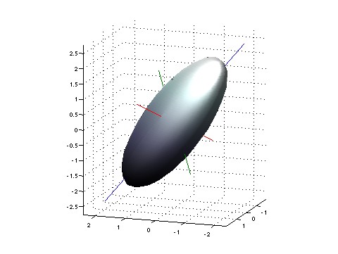
To a first approximation, this cloud will be shaped like a little ellipsoid. And if you can pick the average value of your observables to be whatever you’ll like, you’ll get lots of little ellipsoids this way, one centered at each point. And the cool idea is to imagine the space of possible values of your observables as having a weirdly warped geometry, such that relative to this geometry, these ellipsoids are actually spheres.
This weirdly warped geometry is an example of an ‘information geometry’: a geometry that’s defined using the concept of information. This shouldn’t be surprising: after all, we’re talking about maximum entropy, and entropy is related to information. But I want to gradually make this idea more precise.
Bring on the math!
We’ve got a bunch of observables 


This state
lying in some open subset of 
By the way, I should really call this Gibbs state 

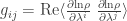
Now at each point

If we take its real part, we get a symmetric matrix:
It’s also nonnegative — that’s easy to see, since the variance of a probability distribution can’t be negative. When we’re lucky this matrix will be positive definite. When we’re even luckier, it will depend smoothly on 
So far this is all review of last time. Sorry: I seem to have reached the age where I can’t say anything interesting without warming up for about 15 minutes first. It’s like when my mom tells me about an exciting event that happened to her: she starts by saying “Well, I woke up, and it was cloudy out…”
But now I want to give you an explicit formula for the metric
Crooks does the classical case — so let’s do the quantum case, okay? Last time I claimed that in the quantum case, our maximum-entropy state is the Gibbs state

where 

(To be honest: last time I wrote the indices on the conjugate variables 

Also last time I claimed that it’s tremendously fun and enlightening to take the derivative of the logarithm of

But now let’s take the derivative of the logarithm of
we get

Next, let’s differentiate both sides with respect to 

Hey! Now we’ve got a formula for the ‘fluctuation’ of the observable

This is incredibly cool! I should have learned this formula decades ago, but somehow I just bumped into it now. I knew of course that 
But I never had the brains to think about 
Now we get our cool formula for
But now that we know

we get the formula we were looking for:
Beautiful, eh? And of course the expected value of any observable 

so we can also write the covariance matrix like this:

Lo and behold! This formula makes sense whenever
Indeed, whenever we have any smooth function from a manifold to the space of density matrices for some Hilbert space, we can define
The classical analogue is the somewhat more well-known ‘Fisher information metric’. When we go from quantum to classical, operators become functions and traces become integrals. There’s nothing complex anymore, so taking the real part becomes unnecessary. So the Fisher information metric looks like this:

Here I’m assuming we’ve got a smooth function 


Crooks says more: he describes an experiment that would let you measure the length of a path with respect to the Fisher information metric — at least in the case where the state 
There’s a lot more to say about this, and also about another question: What use is the Fisher information metric in the general case where the states
But it’s dinnertime, so I’ll stop here.
[Note: in the original version of this post, I omitted the real part in my definition 


There’s an interesting generalization of these ideas in the followup paper:
• Far-From-Equilibrium Measurements Of Thermodynamic Length, E. H. Feng, G.E. Crooks Phys. Rev. E 79, 012104 (2009).
The idea is that we think of the λs as the set of controllable parameters of the system. These could include conjugate variables, such as pressure, or mechanical variables such as volume. If you fix the pressure (or equivalently the average volume) then the volume fluctuates. If you fix the volume the pressure fluctuates. However, with fixed volume the second derivatives of the log partition function are no longer equal to the covariance matrix or Fisher information, but the Fisher information matrix is still equal to the covariance matrix.
I’ll check out that new article — thanks! It’s always pleasing but also a bit scary when the author of a paper I’m discussing shows up to comment. Luckily I mostly discuss papers I enjoyed, and that’s very much the case with the paper of yours I’m discussing here. It may not have been your main goal, but you gave a really quick and lucid explanation of the otherwise mysterious Fisher information metric
Actually, it was my indeed my intention to give a quick and lucid explanation of the otherwise mysterious Fisher information metric. Personally, I always found the idea intriguing, but enigmatic. I reasoned, if Fisher information is so great, why doesn’t it show up in statistical mechanics like entropy does? The answer turns out is that it does; for a Gibbs ensemble the Fisher information matrix is the covariance matrix. I think that’s kind of cool.
I think it’s very cool.
Well, I’ve been reading TWF off and on forever, so the feeling’s mutual.
It is not mysterious: see
http://www.lti.cs.cmu.edu/Research/Thesis/GuyLebanon05.pdf
and especially the wonderful:
http://citeseerx.ist.psu.edu/viewdoc/summary?doi=10.1.1.71.2901
Check out the proofs.
You can also see it as a differential of a Kullback-Leibler divergence between the same parametric probability model:
Great! I’ll use this opportunity to ask a question whose answer is probably too obvious for the experts:
I learned about the Fisher metric from this blog and Wikipedia only, and I would like to know some examples which kind of problems can be solved, and how, with this concept.
In the paper you linked to, you wrote
So I gather that the thermodynamic length can be used to describe driven systems far from equilibrium – is there an example of a “concrete system” that can be studied in this way?
The people who developed thermodynamic length were interested in optimizing macroscopic thermodynamic processes, such as distillation columns, and what not. I’m interested in seeing if we can take those ideas and use them to understand the non-equilibrium behavior of microscopic machines; biological molecular motors, nanoscale solar cells, molecular pores and so on.
For a concrete system I like to think about a single RNA hairpin being pulled apart using optical tweezers, since this is an experiment that can be done today. David Sivak and I are currently writing up a paper where we look at the Fisher information and metric for a (highly simplified) model of this experiment, and how the FI relates to the dissipation.
I wonder how much the frustrations of doing equations on the Web have cumulatively held back the progress of science. . . .
Well, Andrew at some point figured out how to get itex2mml to work on WordPress. This would allow the blog to have the same exact itex capability as the nCafe, nLab, and the nForum.
If you ask him super nicely, he may be able to get it working here.
Here is a test WordPress site that uses itex2mml
Serving MathML
Andrew offered to have the Azimuth blog on a website that did itex2mml, but I’ve always felt that the bother of installing fonts limited the readership of the n-Café. I know plenty of mathematicians who never got around to installing those fonts. Some of them even suffered through n-Café articles interspersed with gobbledygook where there should have been equations, while others (no doubt) just stayed away.
In the case of the n-Café, which was trying to attract a small but committed audience, that was probably okay. But for this blog, the goal of attracting a big audience of people interested in ‘saving the planet’ overshadows the goal of getting really nifty-looking equations.
Of course one might argue that these posts on information geometry, full of equations, do not belong on Azimuth! They may even scare away the eco-minded people I’m trying to attract. Or, they may diffuse the thrust of this blog.
But so far I’ve been hoping these posts attract mathematicians and physicists, who then may become interested in ecological issues. It seems to be working, sort of.
Regarding installed fonts, maybe the latest version might help?
MathJax
With the appearance of informational geometric notions in quantum statistics and machine learning, how should that lead us to answer the question raised in this post as to how much of physical theory is inference? Ariel Caticha, in The Information Geometry of Space and Time, goes so far as “The laws of physics could be mere rules for processing information about nature.”
When someone says something like “The laws of physics could be mere rules for processing information about nature”, the only controversial bit is the word “mere”, which suggests all sorts of deep mysteries, but doesn’t actually explain them.
Caticha’s paper looks interesting, but it’s hard to tell how interesting. It seeks to describe points in space as “merely” labels for probability distributions, getting a Riemannian metric on space which is “merely” the Fisher information metric.
The fun starts when Caticha cooks up a dynamics that describes how the geometry of space evolves in time. This is reminiscent of Wheeler’s “geometrodynamics”: a formulation of Einstein’s equation of general relativity that focuses on how the geometry of space changes with time. Caticha points this out… but alas, leaves open the question of whether his dynamics matches the usual dynamics in general relativity!
If it worked, it would be nice. This would also be a way of sidestepping Eric Forgy’s desire for a Lorentzian metric. I don’t see any way to get a Lorentzian metric from a Fisher information metric: the latter is always Riemannian (i.e., positive definite).
But I think this whole program of getting general relativity from information theory is a bit over-speculative… until someone gets it to work.
For what its worth, I never suggested you could (or that you should even try to) get a Lorentzian metric from the Fisher information metric. What I suggested is what I put forward here. Nothing more nothing less.
The Fisher information metric defines the spatial component of your Lorentzian metric where “space” is the probabilistic space whose length is standard deviation and cosines of angles are correlations.
The “time” component corresponds to the deterministic part of your observable where length corresponds to the mean. It is most easily seen as a differential
where is standard deviation and
  is mean.
The Fisher information metric sees the “spatial” component . The “temporal” component of the metric sees the deterministic part
 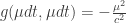 .
.
The full inner product of your observable is then
where is a parameter that relates to “risk aversion” in the financial interpretation.
The mathematics is very neat. The algebra gives meaningful results that have clear statistical meaning.
Often, I would like to print posts from this site, but unfortunately the result is always disastrous; at least in Firefox. Typically the output is a union of the first page of {page header, article, comments, page footer}.
I solve it by copy&paste into OpenOffice and then print. Is there a better way?
Michael
I don’t know! I see what you mean about this problem. Maybe someone else knows more about solutions.
For This Week’s Finds, you’ll probably find it easier to print the version on my website.
[…] suppose we’re working in the special case discussed in Part 2, where our manifold is an open subset of , and at the point is the Gibbs state with . Then all […]
[…] Part 1 • Part 2 • Part 3 • Part 4 • Part […]
[…] found the above in the nice blog of John Baez where Vasileios Anagnostopoulos says about that in the […]