Information Geometry (Part 6)

So far, my thread on information geometry hasn’t said much about information. It’s time to remedy that.

I’ve been telling you about the Fisher information metric. In statistics this is nice a way to define a ‘distance’ between two probability distributions. But it also has a quantum version.

So far I’ve showed you how to define the Fisher information metric in three equivalent ways. I also showed that in the quantum case, the Fisher information metric is the real part of a complex-valued thing. The imaginary part is related to the uncertainty principle.

You can see it all here:

• Part 1 • Part 2 • Part 3 • Part 4 • Part 5

But there’s yet another way to define the Fisher information metric, which really involves information.

To explain this, I need to start with the idea of ‘information gain’, or ‘relative entropy’. And it looks like I should do a whole post on this.

So:

Suppose that $\Omega$ is a measure space — that is, a space you can do integrals over. By a probability distribution on $\Omega$ , I’ll mean a nonnegative function

$p : \Omega \to \mathbb{R}$

whose integral is 1. Here $d \omega$ is my name for the measure on $\Omega$ . Physicists might call $\Omega$ the ‘phase space’ of some classical system, but probability theorists might call it a space of ‘events’. Today I’ll use the probability theorist’s language. The idea here is that

$\int_A \; p(\omega) \; d \omega$

gives the probability that when an event happens, it’ll be one in the subset $A \subseteq \Omega$ . That’s why we want

$p \ge 0$

Probabilities are supposed to be nonnegative. And that’s also why we want

$\int_\Omega \; p(\omega) \; d \omega = 1$

This says that the probability of some event happening is 1.

Now, suppose we have two probability distributions on $\Omega$ , say $p$ and $q$ . The information gain as we go from $q$ to $p$ is

$S(p,q) = \int_\Omega \; p(\omega) \log(\frac{p(\omega)}{q(\omega)}) \; d \omega$

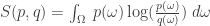
We also call this the entropy of $p$ relative to $q$ . It says how much information you learn if you discover that the probability distribution of an event is $p$ , if before you had thought it was $q$ .

I like relative entropy because it’s related to the Bayesian interpretation of probability. The idea here is that you can’t really ‘observe’ probabilities as frequencies of events, except in some unattainable limit where you repeat an experiment over and over infinitely many times. Instead, you start with some hypothesis about how likely things are: a probability distribution called the prior. Then you update this using Bayes’ rule when you gain new information. The updated probability distribution — your new improved hypothesis — is called the posterior.

And if you don’t do the updating right, you need a swift kick in the posterior!

So, we can think of $q$ as the prior probability distribution, and $p$ as the posterior. Then $S(p,q)$ measures the amount of information that caused you to change your views.

For example, suppose you’re flipping a coin, so your set of events is just

$\Omega = \{ \mathrm{heads}, \mathrm{tails} \}$

In this case all the integrals are just sums with two terms. Suppose your prior assumption is that the coin is fair. Then

$q(\mathrm{heads}) = 1/2, \; q(\mathrm{tails}) = 1/2$

But then suppose someone you trust comes up and says “Sorry, that’s a trick coin: it always comes up heads!” So you update our probability distribution and get this posterior:

$p(\mathrm{heads}) = 1, \; p(\mathrm{tails}) = 0$

How much information have you gained? Or in other words, what’s the relative entropy? It’s this:

$S(p,q) = \int_\Omega \; p(\omega) \log(\frac{p(\omega)}{q(\omega)}) \; d \omega = 1 \cdot \log(\frac{1}{1/2}) + 0 \cdot \log(\frac{0}{1/2}) = 1$

Here I’m doing the logarithm in base 2, and you’re supposed to know that in this game $0 \log 0 = 0$ .

So: you’ve learned one bit of information!

That’s supposed to make perfect sense. On the other hand, the reverse scenario takes a bit more thought.

You start out feeling sure that the coin always lands heads up. Then someone you trust says “No, that’s a perfectly fair coin.” If you work out the amount of information you learned this time, you’ll see it’s infinite.

Why is that?

The reason is that something that you thought was impossible — the coin landing tails up — turned out to be possible. In this game, it counts as infinitely shocking to learn something like that, so the information gain is infinite. If you hadn’t been so darn sure of yourself — if you had just believed that the coin almost always landed heads up — your information gain would be large but finite.

The Bayesian philosophy is built into the concept of information gain, because information gain depends on two things: the prior and the posterior. And that’s just as it should be: you can only say how much you learned if you know what you believed beforehand!

You might say that information gain depends on three things: $p$ , $q$ and the measure $d \omega$ . And you’d be right! Unfortunately, the notation $S(p,q)$ is a bit misleading. Information gain really does depend on just two things, but these things are not $p$ and $q$ : they’re $p(\omega) d\omega$ and $q(\omega) d\omega$ . These are called probability measures, and they’re ultimately more important than the probability distributions $p$ and $q$ .

To see this, take our information gain:

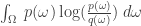
$\int_\Omega \; p(\omega) \log(\frac{p(\omega)}{q(\omega)}) \; d \omega$

and juggle it ever so slightly to get this:

$\int_\Omega \; \log(\frac{p(\omega) d\omega}{q(\omega)d \omega}) \; p(\omega) d \omega$

Clearly this depends only on $p(\omega) d\omega$ and $q(\omega) d\omega$ . Indeed, it’s good to work directly with these probability measures and give them short names, like

$d\mu = p(\omega) d \omega$

$d\nu = q(\omega) d \omega$

Then the formula for information gain looks more slick:

$\int_\Omega \; \log(\frac{d\mu}{d\nu}) \; d\mu$

And by the way, in case you’re wondering, the $d$ here doesn’t actually mean much: we’re just so brainwashed into wanting a $d x$ in our integrals that people often use $d \mu$ for a measure even though the simpler notation $\mu$ might be more logical. So, the function

$\frac{d\mu}{d\nu}$

is really just a ratio of probability measures, but people call it a Radon-Nikodym derivative, because it looks like a derivative (and in some important examples it actually is). So, if I were talking to myself, I could have shortened this blog entry immensely by working with directly probability measures, leaving out the $d$ ‘s, and saying:

Suppose $\mu$ and $\nu$ are probability measures; then the entropy of $\mu$ relative to $\nu$ , or information gain, is

$S(\mu, \nu) = \int_\Omega \; \log(\frac{\mu}{\nu}) \; \mu$

But I’m under the impression that people are actually reading this stuff, and that most of you are happier with functions than measures. So, I decided to start with

$S(p,q) = \int_\Omega \; p(\omega) \log(\frac{p(\omega)}{q(\omega)}) \; d \omega$

and then gradually work my way up to the more sophisticated way to think about relative entropy! But having gotten that off my chest, now I’ll revert to the original naive way.

As a warmup for next time, let me pose a question. How much is this quantity

$S(p,q) = \int_\Omega \; p(\omega) \log(\frac{p(\omega)}{q(\omega)}) \; d \omega$

like a distance between probability distributions? A distance function, or metric, is supposed to satisfy some axioms. Alas, relative entropy satisfies some of these, but not the most interesting one!

• If you’ve got a metric, the distance between points should always be nonnegative. Indeed, this holds:

$S(p,q) \ge 0$

So, we never learn a negative amount when we update our prior, at least according to this definition. It’s a fun exercise to prove this inequality, at least if you know some tricks involving inequalities and convex functions — otherwise it might be hard.

• If you’ve got a metric, the distance between two points should only be zero if they’re really the same point. In fact,

$S(p,q) = 0$

if and only if

$p d\omega = q d \omega$

It’s possible to have $p d\omega = q d \omega$ even if $p \ne q$ , because $d \omega$ can be zero somewhere. But this is just more evidence that we should really be talking about the probability measure $p d \omega$ instead of the probability distribution $p$ . If we do that, we’re okay so far!

• If you’ve got a metric, the distance from your first point to your second point is the same as the distance from the second to the first. Alas,

$S(p,q) \ne S(q,p)$

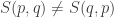
in general. We already saw this in our example of the flipped coin. This is a slight bummer, but I could live with it, since Lawvere has already shown that it’s wise to generalize the concept of metric by dropping this axiom.

• If you’ve got a metric, it obeys the triangle inequality. This is the really interesting axiom, and alas, this too fails. Later we’ll see why.

So, relative entropy does a fairly miserable job of acting like a distance function. People call it a divergence. In fact, they often call it the Kullback-Leibler divergence. I don’t like that, because ‘the Kullback-Leibler divergence’ doesn’t really explain the idea: it sounds more like the title of a bad spy novel. ‘Relative entropy’, on the other hand, makes a lot of sense if you understand entropy. And ‘information gain’ makes sense if you understand information.

Anyway: how can we save this miserable attempt to get a distance function on the space of probability distributions? Simple: take its matrix of second derivatives and use that to define a Riemannian metric $g_{ij}$ . This Riemannian metric in turn defines a metric of the more elementary sort we’ve been discussing today.

And this Riemannian metric is the Fisher information metric I’ve been talking about all along!

More details later, I hope.

This entry was posted on Friday, January 21st, 2011 at 8:02 am and is filed under information and entropy. You can follow any responses to this entry through the RSS 2.0 feed. You can leave a response, or trackback from your own site.

21 Responses to Information Geometry (Part 6)

John Sidles says:

21 January, 2011 at 2:57 pm

John, the two themes of your previous (excellent) essay #5 (namely dissipative physics and partition functions) can be combined with the theme of this essay #6 (namely probability measures) as follows.

Let us consider a spin-j particle in a magnetic field (so that it has equally-spaced energy levels) that is in dynamical contact with a thermal reservoir, so that its relaxation is described by Bloch parameters (so the harmonic oscillator is simply the infinite-j limit). Then unravel the dynamics, by the methods of Carmichael and Caves, in a Lindblad gauge that has no quantum jumps.

Now ask three natural questions: (1) What is the geometric submanifold of Hilbert space onto which the quantum trajectories are dynamically compressed? (2) What is the pulled-back symplectic structure of that submanifold? (3) What is the induced P-representation of the thermal density matrix?

The answers are simple and geometrically natural: (1) The manifold is the familiar Riemann sphere of the Bloch equations. (2) The symplectic structure associated to Bloch flow is canonical symplectic structure of the Riemann sphere. (2) The positive P-representation is given in terms of the thermal Q representation by

$P_{j}(x) = 1/Q_{j+1}(-x).$

These geometric relations are reflections of the general principle that Wojciech Zurek calls einselection … can be verified algebraically, yet the motivation for their derivation arises wholly in geometric ideas associated to Kählerian structure and Hamiltonian/Lindbladian flow.

It is perfectly feasible to systematically translate the whole of Nielsen and Chang’s Quantum Computation and Quantum Information from its original algebraic language into the geometric language of Kählerian/Hamiltonian/Lindbladian flow.

The resulting algebraic and geometric representations of quantum dynamics are rigorously equivalent … and yet they “sit in our brains in different ways” (in Bill Thurston’s phrase). In practical quantum systems engineering both the algebraic and geometric dynamical pictures come into play … it’s fun! :)

Reply
- John Baez says:
  
  24 January, 2011 at 9:46 am
  
  Your comment sounds interesting but there are a lot of things I don’t understand about it, so it’s quite mysterious. Here are a few questions. I could try to look up answers on the all-knowing Google, but it’s probably better for other people if I just ask.
  
  I should probably start with just one. If you answer that, nice and simply, without saying a whole lot of stuff that raises new questions in my mind, I can move on to the next.
  
  You write:
  
  Let us consider a spin-j particle in a magnetic field (so that it has equally-spaced energy levels) that is in dynamical contact with a thermal reservoir, so that its relaxation is described by Bloch parameters (so the harmonic oscillator is simply the infinite-j limit).
  
  I know why a spin-j particle in a magnetic field has (2j+1) equally spaced energy levels. But I don’t know what its “Bloch parameters” are. What are they?
  
  I know about the Bloch sphere for a spin-1/2 particle. Each mixed state has expectation values of angular momentum operators $J_x, J_y, J_z$ lying in some ball. That would also be true for higher spins, though the ball would have a bigger radius. Is that what you’re talking about?
  
  Reply
John Sidles says:

24 January, 2011 at 12:07 pm

Yep! The Bloch parameters are commonly denoted $T_1$ and $T_2$ … in the magnetic resonance literature these are often called the longitudinal and transverse relaxation times. In the infinite-j limit $T_1 = \pi Q/f$ , where $f$ is the harmonic oscillator frequency and $Q$ is the quality. The details are worked out in Spin microscopy’s heritage, achievements, and prospects and references therein.

It is instructive to tell this same story as it might have unfolded in a universe in which quantum systems engineers embraced category theory early and fervently … you can regard the following as the (real-time!) first draft of a lecture that I’ll give at the Asilomar Experimental Nuclear Magnetic Resonance Conference (ENC) this April … comments and corrections are welcome!

We’ll begin by noticing that “Mac Lane has said that categories were originally invented, not to study functors, but to study natural transformations.” (Baez and Dolan, Categorification, 1998). In seeking an original text for this quote, the best that I have found (so far) is Mac Lane’s “But I emphasize that the notions category and functor were not formulated or put in print until the idea of a natural transformation was also at hand.” (Mac Lane, The development and prospects for category theory, 1996). John (B), is there a better text than this one?

Another terrific article by Mac Lane is his Chauvenet Lecture Hamiltonian mechanics and geometry (1970), which closes with the idea that “More use of categorical ideas may be indicated [in dynamics] … . Here, as throughout mathematics, conceptual methods should penetrate deeper to give clearer understanding.”

For engineers, one major obstruction to wider categoric-theoretic applications is that commutative diagrams express equivalences that are exact. Exactitude is wonderful when it reflects exact conservation laws or exact gauge-type invariances. But how can category theoretic methods help us in the case (overwhelmingly more common for engineers) of calculations that are not exact?

One thing we can do is go all the way back to the very first commutative diagram (or is it?) that appeared in the mathematical literature, namely the one in Section 5 of Mac Lane and Eilenberg’s Natural isomorphisms in group theory (1942). We alter it to express not a commutative relation, but rather a projective relation (so that the arrow-heads are cyclic rather commutative). The resulting category-theoretic notion of projective naturality is equally rigorous to the traditional notion of commutative naturality, but less stringent in its implications and thus broader in its applications … this is exactly what engineers need.

The details are worked through in a draft preprint Elements of naturality in dynamical simulation frameworks for Hamiltonian, thermostatic, and Lindbladian flows on classical and quantum state-spaces (arXiv:1007.1958) … Tables I and II recast the commutative diagrams of Eilenberg and Mac Lane into the projective form that is more suited to practical engineering, and the remainder of the preprint systematically translates Chapters 2 and 8 of Nielsen and Chuang’s Quantum Computation and Quantum Information—including the Bloch equations—into this geometric/category-theoretic framework.

We’re now reworking this arXiv:1007.1958 preprint (prior to its presentation at Asilomar) to pay tribute to its category-theoretic origins on the one had, and yet to make clear its rigorous formal equivalence to traditional algebraic formulations of quantum dynamics on the other hand. Hence our desire to reference original texts whenever possible … suggestions from category-theorists in this regard are very welcome.

We have found that many wonderful articles on geometric dynamics are readily appreciated in terms of these category-theoretic ideas. In particular, Ashtekar and Schilling’s Geometrical formulation of quantum mechanics (1999) and J.W. vanHolten’s Aspects of BRST quantization (2005) both are founded upon geometric ideas that are well-expressed in a category-theoretic notation.

One comes away from this reading with the idea that, for practical purposes at least, the effective state-space of quantum mechanics is not a flat, non-dynamic Hilbert space of exponentially large dimensionality, but rather is a curved, dynamical state-space of polynomial dimensionality … very much like the state-space of classical mechanics. This is good news for 21st century mathematicians, scientists, and engineers: it means that there is plenty of both practical and fundamental work to do.

Does nature herself exploit the mathematics of projective naturality to render herself easy to simulate? Is nature’s state-space of quantum dynamics a Hilbert space only in a small-dimension local approximation? That is a fun question—and a great virtue of category-theoretic method is that they allow us to pose this question cleanly.

From an “Azimuthal” point-of-view, the main objective is perhaps more engineering-oriented: to develop 21st century spin metrology methods that “see every atom in its place,” precisely as von Neumann and Feynman once envisioned. What their 20th century envisioned as an utopian capability, our 21st century has reasonable prospects of achieving in practice … and that is exciting.

Reply
- John Baez says:
  
  24 January, 2011 at 12:33 pm
  
  Hmm. You said how the Bloch parameters are denoted, and what they’re called, but not what they are. I guessed that they were the expectation values of $J_x, J_y$ and $J_z$ for a spin-j particle, and you said:
  
  Yep!
  
  but then you just mentioned two things, denoted $T_1$ and $T_2$ … and you said they’re called relaxation times. So I don’t think I understand, yet… and my guess doesn’t sound right.
  
  So: what are the Bloch parameters, exactly? I can’t get into all the fancier stuff you’re discussing before I understand the basics.
  
  We’ll begin by noticing that “Mac Lane has said that categories were originally invented, not to study functors, but to study natural transformations.” (Baez and Dolan, Categorification, 1998). In seeking an original text for this quote, the best that I have found (so far) is Mac Lane’s “But I emphasize that the notions category and functor were not formulated or put in print until the idea of a natural transformation was also at hand.” (Mac Lane, The development and prospects for category theory, 1996). John (B), is there a better text than this one?
  
  That could easily be the best. A quick Google scan reveals that everyone is running around saying a version of the quote sort of like mine, but without giving a source. Perhaps they’re all quoting me!
  
  But I know I got it from somewhere reputable, and maybe it was this… or maybe just verbally, from someone who knew Mac Lane. (I met him a few times, but he didn’t say this to me!)
  
  By the way, you can do LaTeX here if you put ‘latex’ right after the first dollar sign, and don’t do double dollar signs or anything too fancy. Thus,
  
  $latex \int e^x dx = e^x + C$
  
  gives
  
  $\int e^x dx = e^x + C$
  
  I’ve been LaTeXifying some of your comments thus far, just for fun. But this is how one does it oneself.
  
  Reply
John Sidles says:

24 January, 2011 at 1:21 pm

Thank you, John, for the LaTeXing hint!

With regard to the Bloch parameters, the Wikipedia pages on (1) the Bloch equations, (2) the Bloch-Torrey equations, and (3) the Landau-Lifshitz Gilbert (LLG) equations give all the definitions and dynamical equations … but unfortunately the Wikipedia version of the dynamical equations are not expressed in the geometrically natural language of symplectic and metric flow (per your post Information Geometry #5) … this translation one has to do for one’s self.

Ok, so let’s do it. If the Hamiltonian potential associated to the Bloch equation is the usual quantum-state expectation of the Hamiltonian operator on the submanifold of coherent states, then what might be the symplectic form on the Bloch sphere of states? Well, what else could it be … but the canonical $S^2$ volume form?

Guided by this intuition, it is easy to work out that the symplectic/Hamiltonian flow on the Bloch sphere is identical to Wikipedia’s Bloch equations, which with the addition of a metric flow component is identical to the LLG equations, etc. (and we have a student writing up these equivalences).

In other words, the Bloch equations, BLoch-Torrey equations, LLG equations, etc. all are geometrically natural from a category-theoretic point-of-view. Any other result would be wholly unexpected … yet it is remarkable how few textbooks (none AFAICT) discuss the symplectic and metric structures that are naturally associated to Bloch/LLG dynamics.

Reply
- John Baez says:
  
  25 January, 2011 at 2:45 am
  
  So you’re not going to tell me what the Bloch parameters are?
  
  That’s too bad, because it’s just the first of many questions I had, but I can’t really proceed without knowing the answer to this one.
  
  I can of course look things up, but I’m too busy, so I’d been hoping to have a conversation of the old-fashioned sort, where mathematician A says “What are the Bloch parameters?” and mathematician B says “The Bloch parameters are…”
  
  Reply
  - Justin says:
    
    1 February, 2011 at 12:30 am
    
    This is not my expertise per se, but here is the general picture:
    T1 is spin-lattice relaxation time. It is a characteristic time of re-equilibration of spin states responding to thermal fluctuations, leading to thermalization.
    T2 is spin-spin relaxation time. It is a characteristic time of re-equilibration of spin states responding to quantum fluctuations, leading to decoherence.
    
    Reply
John Sidles says:

25 January, 2011 at 1:53 pm

John, I’m really trying … it’s tough to balance rigorous but too-long, against brief but non-rigorous. Here’s another try.

In any linear model of density matrix relaxation, the relaxation is described by a set of rate constants … these rate constants are the Bloch parameters broadly defined.

A particularly common case is a spin-1/2 particle in a magnetic field, whose relaxation is transversely isotropic with respect to the field direction. Then the Bloch relaxation is described by precisely two Bloch parameters … traditionally these parameters are called $T_1$ and $T_2$ , and the canonical reference is Slichter’s Principles of Magnetic Resonance.

Very much more can be said … the discussion of the “Lindblad form” in Nielsen and Chuang Ch. 8.4 is a pretty good start … one has to be ready for the practical reality that different authors—partly by history and partly by practical necessity—embrace very different terminology and notation in describing these ideas.

Reply
John Sidles says:

25 January, 2011 at 3:16 pm

As a followup, once one has a reasonable working grasp on the relaxation of density matrices via Lindblad processes, then a logical next step is to abandon density matrix formalisms … in favor of quantum trajectory formalisms … see in particular the unravelling formalism introduced by Carmichael in his An Open Systems Approach to Quantum Optics (1993) … as far as I know, this is the work that introduced the now-popular concept of “unravelling” to the quantum literature (see Carmichael’s Section 7.4, page 122).

Here the guiding mathematical intuition is that density matrices are not defined on non-Hilbert quantum state-spaces (for example, on tensor network state-spaces) … but unravelled ensembles of trajectories are well-defined … thus the pullback (of dynamical structures) and the pushforward (of trajectories and data-streams) is seen to be geometrically natural … in which respect Carmichael-type quantum unravelling formalisms are more readily generalizable & geometrically natural than density matrix formalisms.

The preceding strategy for making mathematical and physical sense of a vast corpus of literature is driven mainly by considerations of geometric and category-theoretic naturality … no doubt many alternative approaches are feasible … this diversity is what’s fun about quantum dynamics. I hope this helps! :)

Reply
John Sidles says:

26 January, 2011 at 12:54 pm

Continuing the above discussion, on Dick Lipton’s weblog Gödel’s Lost Letter and P=NP, the intimate relation of the above ideas to modern-day (classical) [quantum] {informatic} simulation codes is discussed.

Reply
David Corfield says:

12 February, 2011 at 2:57 pm

I see on the Wikipedia page they write

In this article, this will be referred to as the divergence from P to Q, although some authors call it the divergence “from Q to P” and others call it the divergence “between P and Q” (though note it is not symmetric as this latter terminology implies).

Still it seems odd where you write

The information gain as we go from $p$ to $q$ is …,

I think I’d prefer it the other way around.

Later you write

So, relative entropy does a fairly miserable job of acting like a distance function.

There’s an argument that relative entropy is the square of a distance, agreed a few comments below. Look for Pythagorean theorem in Elements of Information theory here.

Reply
- John Baez says:
  
  13 February, 2011 at 9:34 am
  
  David wrote:
  
  Still it seems odd where you write
  
  The information gain as we go from $p$ to $q$ is …
  
  I think I’d prefer it the other way around.
  
  Oh, definitely! That was just a typo — I’ve fixed it now, thanks. I should mind my $p$ ‘s and $q$ ‘s.
  
  There’s an argument that relative entropy is the square of a distance, agreed a few comments below.
  
  Only after you symmetrize it, of course. The relative entropy is not symmetric:
  
  $S(p,q) \ne S(p,q)$
  
  so it can’t give a metric (of the traditional symmetric sort) when you take its square root. But Suresh Venkat is claiming that the symmetrized gadget, which he calls the ‘Jensen-Shannon distance’:
  
  $\frac{1}{2} S(p,q) + \frac{1}{2} S(q,p)$
  
  does give a metric when you take its square root. I’ll have to check this, or read about it somewhere if I give up. You just need to check the triangle inequality… the rest is obvious.
  
  But as your n-Café comment notes, there’s also another nice metric floating around. If we define a version of relative entropy based on Rényi entropy instead of the usual Shannon kind, we get something called the ‘Rényi divergence’ which is symmetric only for the special case $\alpha = 1/2$ … and while it still doesn’t obey the triangle inequality in that case, it’s a function of something that does. Not-so-coincidentally, I was just reading about this today. This thesis has a nice chapter on Rényi entropy and the corresponding version of relative entropy:
  
  • T. A. L. van Even, When Data Compression and Statistics Disagree: Two Frequentist Challenges For the Minimum Description Length Principle, Chap. 6: Rényi Divergence, Ph.D. thesis, Leiden University, 2010.
  
  Yeah, it’s on page 179:
  
  Only for $\alpha = 1/2$ is Rényi divergence symmetric in its arguments. Although not itself a metric, it is a function of the square of the Hellinger distance
  
  $\mathrm{Hel}^2(p,q) = \sum_{i = 1}^n (\sqrt{p_i} - \sqrt{q_i})^2$
  
  [Gibbs and Su, 2002].
  
  Anyway, my goal in this post was pretty limited. I just wanted to explain the concept of relative entropy a little bit, so people can following what I’m saying when I explain how it’s related to the Fisher information metric.
  
  Reply
Information Geometry (Part 7) « Azimuth says:

2 March, 2011 at 2:40 am

Now I want to describe how the Fisher information metric is related to relative entropy […]

Reply
Information Geometry (Part 8) « Azimuth says:

26 May, 2011 at 10:09 am

Remember what I told you about relative entropy […]

Reply
Information Geometry (Part 11) « Azimuth says:

7 June, 2012 at 10:00 am

For more on relative entropy, read Part 6 of this series […]

Reply
Luisberis Velazquez says:

22 March, 2013 at 3:14 am

To my knowledge, the notion of relative entropy:

$S(p,q)= -\int \left[d\mu(x)/d\nu(x)\right]\log\left[d\mu(x)/d\nu(x)\right]d\nu(x)$

was early proposed by Jaynes to extend the notion of information entropy to the framework of continuous distributions. However, I think that the relative entropy is not a fully satisfactory generalization of this concept. A natural question here is how to introduce the measure:

$d\nu(x)=q(x)dx$

when no other information is available, except the continuous distribution:

$d\mu(x)=p(x)dx.$

Recently, I proposed a way to overcome this difficulty in the framework of Riemannian geometry of fluctuation theory:

http://iopscience.iop.org/1751-8121/45/17/175002/article

This geometry approach introduces a distance notion:

$ds^{2}=g_{ij}(x)dx^{i}dx^{j}$

between two infinitely close points $x$ and $x+dx$ , where the metric tensor is obtained from the probability density $p(x)$ as follows:

$g_{ij}=-\frac{\partial^{2}\log p}{\partial x^{i}\partial x^{j}}+ \Gamma^{k}_{ij}\frac{\partial\log p}{\partial x^{k}} +\frac{\partial\Gamma^{k}_{jk}}{\partial x^{i}}-\Gamma^{k}_{ij}\Gamma^{l}_{kl}$ .

Here, the symbol $\Gamma^{k}_{ij}$ denote the Levi-Civita affine connections. Formally, this is a set of covariant partial differential equations of second order in terms of the metric tensor. The measure $d\nu(x)$ can be defined as follows:

$d\nu(x)=\sqrt{\left|g_{ij}(x)/2\pi \right| }dx.$

Apparently, the relative entropy that follows from this ansatz is a global measure of the curvature of the manifold $\mathcal{M}$ where the continuous variables $x$ are defined. Some preliminary analysis suggest that curvature $R(x)$ is closely related to the existence of irreducible statistical correlations among the random variables $x$ , that is, statistical correlations that survive any coordinate transformations $y=\phi(x)$ .

Reply
- John Baez says:
  
  22 March, 2013 at 5:46 pm
  
  Hi! How are you constructing your Levi-Civita connection starting from $p?$ I know how to construct a Levi-Civita connection starting from a metric, but you’ve defined your metric starting from a Levi-Civita connection. The fact that you speak of ‘the’ Levi-Civita connection makes me a little nervous, since there are many.
  
  Reply
Luisberis Velazquez says:

22 March, 2013 at 3:18 am

By the way, this is a great blog!

Reply
- John Baez says:
  
  22 March, 2013 at 5:53 pm
  
  Thanks!
  
  Reply
Luisberis Velazquez says:

22 March, 2013 at 8:31 pm

Levi-Civita affine connections or the metric connections only depend on the metric tensor:
$\Gamma _{ij}^{k}\left( x|\theta \right) =g^{km}(x|\theta)\frac{1}{2}\left[\frac{\partial g_{im}(x|\theta)}{\partial x^{j}}+\frac{\partial g_{jm}(x|\theta)}{\partial x^{i}}-\frac{\partial g_{ij}(x|\theta)}{\partial x^{m}}\right]$ ,
and they are the only affine connections with a tonsion-less covariant derivative $D_{k}$ that obeys the condition of Levi-Civita parallelism:
$D_{k}g_{ij}(x)=0$ .
The relation between the metric tensor and the probability density represents a set of covariant partial equations of second-order in terms of the metric tensor. This equation is non-linear and self-consistent. As expected, it is difficult to solve in most of practical situations. However, this ansatz allows to introduce a measure $d\nu(x)$ for the relative entropy only considering the probability density of interest.

Surprinsingly, the value of this relative entropy can be expressed in an exactly way as follows:
$S(p|q)=\log Z-n/2$ ,
where $n$ is the dimension of the manifold $\mathcal{M}$ and $Z$ a certain normalization constant. Precisely, a direct consequence of this set of covariant differential equations is the possibility to rewrite the original distribution function:
$d\mu(x)=p(x)dx$
as follows:
$d\mu(x)=\frac{1}{Z}\exp\left[-\frac{1}{2}\ell^{2}(x,\bar{x})\right]d\nu(x)$ .
Here, $d\nu(x)$ is the invariant measure:
$d\nu(x)=\sqrt{\left| g_{ij}(x)/2\pi \right|}dx$ ;
$\bar{x}$ denotes the most likely point of the distribution, while $\ell^{2}(x,\bar{x})$ denotes the arc-length of geodesics that connects the points $x$ and $\bar{x}$ . Formally, this is a Gaussian distribution defined on a Riemannian manifold $\mathcal{M}$ . The normalization constant $Z$ is reduced to the unity if the manifold $\mathcal{M}$ is diffeomorphic to the n-dimensional Euclidean real space $\mathbb{R}^{n}$ , and it takes different values when the manifold exhibits a curved geometry. Consequently, this type of relative entropy is a global measure of the curvature of the manifold $\mathcal{M}$ where the random variables $x$ are defined. To my present understanding, curvature accounts for the existence of irreducible statistical correlations, something analogous to the irreducible character of gravity in different references frames due to its connection with curvature.

Reply
Luisberis Velazquez says:

22 March, 2013 at 9:03 pm

Sorry with type-errors. The symbol $\theta$ in the Levi-Civita connections comes from my original work, with deals with parametric family of continuous distributions with a number $m$ of shape parameters $\theta=(\theta^{1},\theta^{2},\ldots \theta^{m})$ . Certainly, most of differential equations of Riemannian geometry are difficult to solve. I spend a lot of time (years) to decide to explore this type of statistical geometry. Recently, I realize that some mathematical derivations are not difficult to perform despite the exact mathematical form of the metric tensor $g_{ij}(x)$ is unknown for a concrete distribution $d\mu(x)=p(x)dx$ .

My fundamental interest on this geometry are its applications on classical statistical mechanics. This type of geometry was inspired on Ruppeiner’s geometry of thermodynamics. The metric tensor of this last formulation was modified replacing the usual derivative $\partial_{i}$ by the Levi-Civita covariant derivative:
$g_{ij}(x)=-D_{i}D_{j}\mathcal{S}(x)$ .
Here, $\mathcal{S}(x)$ is the thermodynamic entropy. Since the entropy is a scalar function, the above relation guarantees the covariance of the metric tensor. Moreover, the thermodynamic entropy $\mathcal{S}(x)$ enters in mathematical expression of Einstein postulate of classical fluctuation theory, which should be extended as follows:
$d\mu(x)=\exp\left(\mathcal{S}(x)\right)d\nu(x)$
to guarantee the scalar character of the entropy. The gaussian distribution that I commented above is an exact improvement of gaussian approximation of classical fluctuation theory of statistical mechanics.

Reply

You can use Markdown or HTML in your comments. You can also use LaTeX, like this: $latex E = m c^2 $. The word 'latex' comes right after the first dollar sign, with a space after it. Cancel reply

This site uses Akismet to reduce spam. Learn how your comment data is processed.

	John Tromp on The Busy Beaver Game
	Wolfgang on Protonium
	Giampiero Campa on Agent-Based Models (Part …
	John Baez on Agent-Based Models (Part …
	Paul Pukite (@whut) on Agent-Based Models (Part …
	bhaugen on Agent-Based Models (Part …
	John Baez on Agent-Based Models (Part …
	William Waites on Agent-Based Models (Part …
	John Baez on Agent-Based Models (Part …
	John Baez on Agent-Based Models (Part …

Azimuth