Now for the fun part. Let’s see how tricks from quantum theory can be used to describe random processes. I’ll try to make this post self-contained. So, even if you skipped a bunch of the previous ones, this should make sense.
You’ll need to know a bit of math: calculus, a tiny bit probability theory, and linear operators on vector spaces. You don’t need to know quantum theory, though you’ll have more fun if you do. What we’re doing here is very similar… but also strangely different—for reasons I explained last time.
Rabbits and quantum mechanics
Suppose we have a population of rabbits in a cage and we’d like to describe its growth in a stochastic way, using probability theory. Let 


The variable 
However, there’s a good reason for this trick. We can define two operators on formal power series, called the annihilation operator:

and the creation operator:

They’re just differentiation and multiplication by 

If we then apply the creation operator, we obtain

Voilà! One more rabbit!

The annihilation operator is more subtle. If we start out with
and then apply the annihilation operator, we obtain

What does this mean? The 
The creation and annihilation operators don’t commute:

so for short we say:

or even shorter:
where the commutator of two operators is
![[S,T] = S T - T S](https://s0.wp.com/latex.php?latex=%5BS%2CT%5D+%3D+S+T+-+T+S+&bg=ffffff&fg=333333&s=0&c=20201002)
The noncommutativity of operators is often claimed to be a special feature of quantum physics, and the creation and annihilation operators are fundamental to understanding the quantum harmonic oscillator. There, instead of rabbits, we’re studying quanta of energy, which are peculiarly abstract entities obeying rather counterintuitive laws. So, it’s cool that the same math applies to purely classical entities, like rabbits!
In particular, the equation ![[a, a^\dagger] = 1](https://s0.wp.com/latex.php?latex=%5Ba%2C+a%5E%5Cdagger%5D+%3D+1&bg=ffffff&fg=333333&s=0&c=20201002)
But how do we actually use this setup? We want to describe how the probabilities

Then, we write down an equation describing the rate of change of 
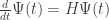
Here 
Catching rabbits

Last time I told you what happens when we stand in a river and catch fish as they randomly swim past. Let me remind you of how that works. But today let’s use rabbits.
So, suppose an inexhaustible supply of rabbits are randomly roaming around a huge field, and each time a rabbit enters a certain area, we catch it and add it to our population of caged rabbits. Suppose that on average we catch one rabbit per unit time. Suppose the chance of catching a rabbit during any interval of time is independent of what happened before. What is the Hamiltonian describing the probability distribution of caged rabbits, as a function of time?
There’s an obvious dumb guess: the creation operator! However, we saw last time that this doesn’t work, and we saw how to fix it. The right answer is

To see why, suppose for example that at some time 

Then the master equation says that at this moment,

Since 


while all the rest have zero derivative at this moment. And that’s exactly right! See, 

Puzzle 1. Show that with this Hamiltonian and any initial conditions, the master equation predicts that the expected number of rabbits grows linearly.
Dying rabbits

Don’t worry: no rabbits are actually injured in the research that Jacob Biamonte is doing here at the Centre for Quantum Technologies. He’s keeping them well cared for in a big room on the 6th floor. This is just a thought experiment.
Suppose a mean nasty guy had a population of rabbits in a cage and didn’t feed them at all. Suppose that each rabbit has a unit probability of dying per unit time. And as always, suppose the probability of this happening in any interval of time is independent of what happens before that time.
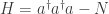
What is the Hamiltonian? Again there’s a dumb guess: the annihilation operator! And again this guess is wrong, but it’s not far off. As before, the right answer includes a ‘correction term’:

This time the correction term is famous in its own right. It’s called the number operator:

The reason is that if we start with
Let’s see why this guess is right. Again, suppose that at some particular time
Then the master equation says that at this time

So, our probabilities are changing like this:


while the rest have zero derivative. And this is good! We’re starting with
Puzzle 2. Show that with this Hamiltonian and any initial conditions, the master equation predicts that the expected number of rabbits decays exponentially.
Breeding rabbits

Suppose we have a strange breed of rabbits that reproduce asexually. Suppose that each rabbit has a unit probability per unit time of having a baby rabbit, thus effectively duplicating itself.
As you can see from the cryptic picture above, this ‘duplication’ process takes one rabbit as input and has two rabbits as output. So, if you’ve been paying attention, you should be ready with a dumb guess for the Hamiltonian: 
But you should also suspect that this dumb guess will need a ‘correction term’. And you’re right! As always, the correction terms makes the probability of things staying the same go down at exactly the rate that the probability of things changing goes up.
You should guess the correction term… but I’ll just tell you:
We can check this in the usual way, by seeing what it does when we have

That’s good: since there are
Puzzle 3. Show that with this Hamiltonian and any initial conditions, the master equation predicts that the expected number of rabbits grows exponentially.
Dueling rabbits
Let’s do some stranger examples, just so you can see the general pattern.

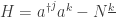
Here each pair of rabbits has a unit probability per unit time of fighting a duel with only one survivor. You might guess the Hamiltonian 

Let’s see why this is right! Let’s see what it does when we have

That’s good: since there are 
(If you prefer unordered pairs of rabbits, just divide the Hamiltonian by 2. We should talk about this more, but not now.)
Brawling rabbits

Now each triple of rabbits has a unit probability per unit time of getting into a fight with only one survivor! I don’t know the technical term for a three-way fight, but perhaps it counts as a small ‘brawl’ or ‘melee’. In fact the Wikipedia article for ‘melee’ shows three rabbits in suits of armor, fighting it out:

Now the Hamiltonian is:

You can check that:

and this is good, because 

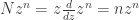
The general rule
Suppose we have a process taking 


I hope you can guess the Hamiltonian I’ll use for this:

This works because

so that if we apply our Hamiltonian to

See? As the probability of having 

Since we can apply functions to operators as well as numbers, we can write our Hamiltonian as:
Kissing rabbits

Let’s do one more example just to test our understanding. This time each pair of rabbits has a unit probability per unit time of bumping into one another, exchanging a friendly kiss and walking off. This shouldn’t affect the rabbit population at all! But let’s follow the rules and see what they say.
According to our rules, the Hamiltonian should be:
However,

and since 

so in fact:

That’s good: if the Hamiltonian is zero, the master equation will say

so the population, or more precisely the probability of having any given number of rabbits, will be constant.
There’s another nice little lesson here. Copying the calculation we just did, it’s easy to see that:

This is a cute formula for falling powers of the number operator in terms of annihilation and creation operators. It means that for the general transition we saw before:
we can write the Hamiltonian in two equivalent ways:

Okay, that’s it for now! We can, and will, generalize all this stuff to stochastic Petri nets where there are things of many different kinds—not just rabbits. And we’ll see that the master equation we get matches the answer to the puzzle in Part 4. That’s pretty easy. But first, we’ll have a guest post by Jacob Biamonte, who will explain a more realistic example from population biology.


For puzzle 1, you have shown for the basis element , that
  and
and  . So the rate of increase of the expected number is
  . So for a general distribution, the rate of increase of the expected number of rabbits is
  .
.
Is there a slick way of doing it via evaluated at
  ?
?
Great! Thanks, David! I have a slick way to do these, but I like your way because, unlike mine, it doesn’t convey the impression that you need to be a crazed quantum physicist to solve these problems.
Here’s my way. We start with some general useful observations that have nothing to do with this particular puzzle. They’ll come in handy for all these puzzles.
As you note, the expected value of the number of rabbits in any probability distribution is
is
On the other hand:
So, if we evaluate at
at  we get the expected number of rabbits:
Now suppose our probability distribution and thus
  depend on time. Then to see how the expected number of rabbits changes with time, we can compute
Let’s try. The old “do whatever you can do” strategy is always good in this sort of situation:
where in the first step we pass the derivative through the linear operator (anyone who doubts we can, belongs in math grad school), and in the second we use the master equation
What can we do next? Well, we can use the definition of (which depends on which puzzle we’re doing) and the definition of
  (which doesn’t):
To solve Puzzle 1, we should show the rate at which the expected number of rabbits grows is a constant. In fact you’ve already shown this constant equals 1, so we know what we’re aiming for.
In this puzzle we have
so the rate at which the expected number of rabbits grows is
and we’re trying to show this equals 1.
But remember that is multiplication by
  , while
This should do the job somehow… no?
All this may seem like overkill—and indeed it is for this puzzle. But it’s a powerful strategy, and after we codify it a bit, it will become less work.
That last equation is where I reached. I guess there was never going to be a simplification before setting . The other two puzzles work out fine.
Great. But that kind of remark tends kill off anyone else’s desire to solve the puzzles: there’s this guy out there who’s already done ’em…
I want to actually see the solutions. I haven’t actually done them. Should I offer a bounty?
My chances of having lengthy stretches of Latex working without preview are slim, but here goes.
Puzzle 2:
so
So, .
.
Great! I don’t mind fixing up the LaTeX around here. You got exponential growth instead of exponential decay, by dropping a minus sign, but that’s no big deal.
Let me try it my way. It’s really the same as your way, just with slightly different notation. Like many physicists I’ve spent decades playing with many different formalisms for operators in quantum field theory, so I can’t resist trying different formalisms for this probabilistic version.
In my general formalism I like to use to mean the total integral of a function over some measure space, so that ‘states’, that is probability distributions, are the functions obeying
and
In the examples today the integral is really a sum, and it might be confusing to use integral notation since we’re using derivatives for a completely different purpose. So let me define sum notation as follows:
This may annoy you, since after all we really have
but please humor me.
So, there’s a nice rule, easily verified:
I mentioned it before: it’s part of the creation operator being a stochastic operator. This implies another nice rule:
Indeed:
The expected value of any observable in the state
  is
is
So, if we’re trying to work out the time derivative of the expected value of , we can start by doing
and then write and
and  using annihilation and creation operators and use our rules.
For example, in Puzzle 2 we have
and the observable we’re interested in is the number of rabbits
so we want to understand
So far I’ve just gotten to the third line of our answer! But I’m having fun playing with the machinery.
Now every kid who’s studied quantum field theory knows
It’s easy to prove, and it says that annihilating a particle and then counting them is the same as counting them, subtracting one and then annihilating one.
So:
but here our rules come in handy!
so we we see
as was to be shown.
Perhaps this fascination with formalism seems odd, but I keep enjoying how everything compares with quantum mechanics! For example, in quantum mechanics the expected value of an observable is
and its time derivative is
hence the vast appeal of Lie algebras. Now the expected value is
and its time derivative is just
We don’t get two terms because shows up just once in the formula — we’re using
  instead of
  . So everything is similar… but eerily simple!
Now you’ve dropped the minus sign too!
Yup. I caught that while you were writing your comment. And I added a bunch of new stuff. Moderator’s privilege, sorry.
Anyway, someone else should try Puzzle 3, to try out the spiffy new modifications of quantum theory!
Why does
Let me try again:
so
but
and for the same reason
so two terms cancel and we’re left with
as desired.
I knew what answer I wanted, so I wasn’t gonna let a few mistakes stop me from getting it!
Thanks, David. But I think all the mathematicians and physicists out there should be ashamed to be lurking in the background while a philosopher is doing all the hard work here.
I’m a little confused about the second line above. Unless I’m missing something
If , then what rewriting makes this
  rather than
  ?
?
Sorry. I didn’t see the equivalence of immediately below the line you mentioned.
What’s quickest for 3? Something like
Then
In english it’s called a truel, but I would prefer it as in German, triel. I know of two western films with truels: The Good, the Bad and the Ugly of which I have forgotten the triel scene, and another good western whose title I’ve forgotten, but remember the paradigmatic triel scene (one character was a poker player)… Sigh, my swiss cheese brain.
I guess the quantum and octonion philosopher has more to say of why its not the duel what makes the world move, but the truel…
BTW I got interested in that stuff because I once worked for the inventor of a 3-player chess variant. (Mess and design of that page is not my fault….). Now I know why I always found duel-chess boring – and methinks it actually makes stupid…
Seems to me we are either in the process of total revolution or meddling in things of the devil — or both! “All seriousness aside”, as once said, Newton and Maxwell/Faraday asserted that there was a continuum of “forces” in the universe, albeit under the aegis of the “field” concept in the latter case. Einstein made the most of this in his remarkable “warping” of space-time dimensional parameters we use to converse about nature. Now, under the province of field operators and commutators we discover maybe all of the universe is ‘quantized’, where integers come to the fore. However, importantly and certainly fortuitously, in physics and perhaps everywhere there exists an inherent “correspondence” in the “classical limit” to the original continuum. All very well, except that the ‘limit’ is apparently only for experimental verification, whereas the quantum picture is what’s “really happening”, except that according to Bohr and Feynman, we don’t ‘understand’ what’s happening!
The mathematical tricks involving differentiation and other operations as enlighteningly shown above are the mechanism behind all this quantization, but except for the various eponyms involved, what, really, are we doing when carrying out this revolution (or diabolical collusion)?
My original venerable antique Leonard Schiff-era QFT background probably accounts for my ignorance here, but I feel there has to be a fairly clear path to just a few fundamental and universally relevant premises that, at least insofar as simply logic is concerned (perhaps abandoning any hope for “common sense”), we substantively know what IS the revolutions. (Which for good measure, according to another post might be involved with the coding of the very life process besides.)
Jack wrote:
Since I don’t really believe in the devil, I guess it must be a revolution!
Seriously: in my former life as a mathematical physicist mainly concerned with ‘foundational’ issues like quantum gravity, I spent a lot of time wondering what quantum theory was trying to tell us. And I wrote a lot about this, too. It’s hard to write about these things without descending into flakiness, unless one uses lots of math as a kind of cold-water cure. So, most of my thoughts are camouflaged under thick layers of math.
If you go here, you’ll see me arguing that to reach a deeper understanding of quantum theory and spacetime, we must exploit the fact that these two columns are mathematically a lot more similar than we tend to give them credit for being:
SPACETME PROCESS
We tend to describe states of matter quantum-mechanically as vectors in a Hilbert space, while also thinking of these states as ‘living in space’ at a given time. We tend to describe quantum-mechanical processes using operators between Hilbert spaces, while also thinking of these processes as ‘living in spacetime’. But from work on quantum gravity, one of the few things that seems really is that space itself must have a quantum state, and spacetime itself must be a quantum process.
As Wheeler put it: in general relativity, spacetime stops being the mere stage on which events play out, and becomes one of the actors. But we also know the actors are quantum-mechanical. So we need a theory of quantum spacetime.
This sounds scary, but luckily there are lots of mathematical clues to point the way. The paper I just linked to lists some. This one lists a lot more:
• John Baez and Aaron Lauda, A prehistory of n-categorical physics, to appear in Deep Beauty: Mathematical Innovation and the Search for an Underlying Intelligibility of the Quantum World, ed. Hans Halvorson, Cambridge U. Press.
When we’re done figuring this out, I’m sure the world will make a lot more sense… though it won’t be ‘common sense’.
But now I’m trying to think about slightly more practical issues. So in this series of posts, I’m taking some of the math developed for the purposes of understanding quantum theory (so-called groupoidification), and reusing a tiny piece of it to think about stochastic processes.
I’m trying to relate what I know about using probability generating functions to the physics formalism. Now John has presented “creation” as an operator. Another way of looking at it is using, for two pgf’s for
for  and
and  and
and  , then the pgf of
  is
is  . So we get the same answer by taking
  (via
(via  ) as the current distribution and
  as the distribution with “definitely exactly one rabbit” (ie
  ).
).
The corresponding rule for is
is  , so (assuming we’re fine with a probability distribution including a value of -1 when we initially had no rabbits) the same calculation gives
  for this. So there’s a difference between annihilating a rabbit and “subtracting a rabbit”. I can see intuitively the difference, because it’s due to the selection of which rabbit dies, but is there a more clear rule for demarcating which cases count as “annihilation” and which count as “subtraction”?
Hi, David!
It sounds like you understand what’s going on, but would like to see it formalized a bit better. Perhaps you’ll feel better if I provide some reassurance that this is a known issue. The question is whether you want to say there are different ways to annihilate one of
  things, or just one way. The problem at hand determines which answer is right.
In combinatorics they distinguish between two types of generating functions: so-called ordinary generating functions:
and so-called exponential generating functions:
(Writing on the left here instead of just
  should be enough to drive Giampiero Campara insane; even I can’t stand it, because
  is just a dummy variable on the right-hand side: these generating functions are not really functions of
  . But the combinatorists have a good reason for this abuse of notation: there is no standard name for the sequence
  , say, except
  .)
.)
In these notes I’ve been using ordinary generating functions. If you differentiate one of these, a factor of shows up:
That suits my applications. If you don’t want that factor of to show up here, you can use exponential generating functions:
But you pay a price: multiplying an exponential generating function by introduces a factor of
  , while this doesn’t happen for ordinary generating functions. Again, ordinary generating functions do the right thing for my applications.
If you don’t want this factor of either way, and you don’t want to introduce any ugly ad hoc rules, I think you’re forced to allow negative numbers of things as well as positive numbers of things. Then instead of a formal power series we can use a Laurent series
As you note, multiplying or dividing this Laurent series by shifts it without introducing any factor of
  either way:
I’ve generally avoided this trick because I’m somewhat confused about the mathematical status of ‘sets with a negative number of elements’, a mysterious topic that has spawned many interesting papers. In physics, when you have one antiparticle, that may perhaps count as having -1 particles, and that’s one reason why negative sets would be nice. But in biology, I see no application of antirabbits. Chemistry is an interesting borderline case: antihydrogen exists, but you won’t find it in your typical child’s chemistry set. Good thing, too.
For vastly more about these issues, see Wilf’s Generatingfunctionology and my page on the mysteries of counting.
And by the way: in case anyone is confused by the fact that differentating (‘annihilating one rabbit’) changes to
to  here, instead of
  :
:
don’t worry: it only took me 10 years to feel perfectly comfortable with this. It’s basically the same effect as when you’re riding a train: the scenery looks like it’s moving backwards, but it’s because you’re moving forwards.
It’s more that I can see what’s happening mathematically, but I’m trying to figure out why, and in what “application” situations, it’s annihilation or subtraction. I’ve been pondering this and I think that it’s this: the sum becomes product of pgf’s is actually only valid for independent variables. And it’s a coincidence that increasing the number of rabbits in a distribution by one is a sum of two independent distributions as well as a transformation of one pgf. So there’s no a priori reason to believe that removing a rabbit is expressible as a difference of two independent distributions, and it doesn’t look like it is expressible that way at all. So given a situation to analyse I guess it’s a case of figuring out if all the operations you’re modelling are combining two independent distributions or transforming one distribution.
The Laurent series example has raising and lowering operators that commute, which ties in, though I’m not sure how loosely, with my paper showing that the quantized complex Klein-Gordon field is empirically equivalent to a Klein-Gordon random field, EPL 87 (2009) 31002.
Dollars in a bank account seem to match the Laurent series model, where there’s exactly one way both to add or to remove one dollar, there aren’t $n$ ways to remove a dollar, and one can be in debt? Must read Wilf’s page and yours on generating functions.
Incidentally, your RSS feed seems not to be working (at least not from Mozilla or Thunderbird).
Shouldn’t it be
Yes, thanks!
I put clearly explained (?) answers to all 3 puzzles at the bottom of this page on my website:
• Network Theory (Part 6).
This page uses jsmath to put LaTeX on a webpage. I think jsmath takes a while to grab the necessary math fonts if you don’t have them. So, while I can link directly to the correct location on the page, the page then expands and I’m left at another location—at least using Firefox 3.6.16 without the math fonts installed. I’d be curious what happens to you!
It might help the reader if you took David T’s point and put in an extra line.
I rewrote the explanation so that future David T’s wouldn’t be confused, but it seems my new explanation was confusing in other ways – more below on that.
I mean as you have it, you’ve already used Rule 2 when you write
Why not write
I wasn’t using Rule 2, I was using the commutation relations and then making a typo, which gave
  .
.
I think the typos are mostly gone now, thanks to you. The more important problem here is that there are so many ways to use the rules to do these calculations that it’s hard to find the ‘best’ way.
Then you have
The second in the first term should be
  .
.
And is it obvious that ? It’s true, but it’s not by Rule 2, unless you strengthen that to
  for all
David C. wrote:
Thanks – fixed!
Rule 2 (for those not keeping score) says
but surely it was clear that this rule applies to all formal power series , even those that happen to be called
  .
.
Well, okay: it obviously wasn’t clear. I’ll make it clearer.
This is how all papers and books should be written: with an audience of actual people reading it as it’s written, saying what they like, what they don’t like, and what they find confusing. Otherwise it’s too easy for author to dream up perfectly convincing reasons that the audience should like or understand something. But if they don’t, they don’t!
Where you have
you need brackets around . And again in the next line.
Thanks. I decided to switch to an argument that seems a bit simpler:
Why are we considering all the s to appear on the left side of all the
  s in H (
 )?
)?
Surely, there can be situations when the order is not- all inputs, then all outputs. Suppose that 2 rabbits meet and fight and one gets killed. The overconfident victor then challenges any one of the remaining rabbits to a duel and one of them then gets killed. The new victor seeing that he might get killed if he further challenges, stops. If this constitutes the transition, shouldn’t H be ?
?
Also, if operating with a on includes n, the number of ways a rabbit can be chosen from n rabbits, then shouldn’t operating with
  also include the number of ways an output rabbit can be chosen from the k inputs?
Arjun wrote:
Because each transition in a stochastic Petri net describes a processes where a bunch of things get used simultaneously to create some other bunch of things.
That’s true. I would think of this using a Petri net with a set consisting of several states. For example: ordinary rabbits, and ‘overconfident victor rabbits’, and ‘wisely cautious victor rabbits’. I’d also introduce several transitions in
  , for example:
ordinary rabbit + ordinary rabbit overconfident victor rabbit
overconfident victor rabbit + ordinary rabbit wisely cautious rabbit
You can try to work out the Hamiltonian for such a process.
Or, you can check to see if the Hamiltonian you propose is an infinitesimal stochastic operator. If it is, it describes some random process. If not, there’s something wrong with it.
Also, if operating with a on includes
  , the number of ways a rabbit can be chosen from n rabbits, then shouldn’t operating with
  also include the number of ways an output rabbit can be chosen from the
  inputs (at least in some cases)?
We shouldn’t redefine it’s too beautiful to change. If we have a situation where a transition occurs at a rate proportional to
  because we need to make some choice among the
  inputs, we can multiply the Hamiltonian by
  to account for that. I don’t think duels between rabbits occur twice as fast because there are 2 choices of which rabbit might survive.
In the section on Dueling Rabbits, you say “(If you prefer unordered pairs of rabbits, just divide the Hamiltonian by 2. We should talk about this more, but not now.)”. Have you talked about this in some later post?
I never got around to it. But it’s easy to create a number of variants of the rate equation and master equation, depending on whether one is interested in:
• ordered k-tuples of not-necessarily-distinct inputs
• unordered k-tuples of not-necessarily-distinct inputs
• ordered k-tuples of distinct inputs
• unordered k-tuples of distinct inputs
In my notes I’m always considering ordered k-tuples of distinct inputs. These are counted by the falling powers This case turns out to be most easily described using annihilation and creation operators. However, to count unordered k-tuples of distinct inputs, you just divide by
  . So, you can just divide each term in the Hamiltonian by a suitable factor.