Globular

One of my goals is to turn category theory, and even higher category theory, into a practical tool for science. For this we need good scientific ideas—but we also need good software.

My friend Jamie Vicary has been developing some of this software, together with Aleks Kissinger and Krzysztof Bar and others. Jamie demonstrated it at the Simons Institute workshop on compositionality. You can watch his demonstration here:

But since Globular runs on a web browser, you can also try it out yourself here:

• Globular.

You can see his talk slides:

• Jamie Vicary, Data structures for quasistrict higher categories. (Talk slides here.)

Abstract. Higher category theory is one of the most general approaches to compositionality, with broad and striking applications across computer science, mathematics and physics. We present a new, simple way to define higher categories, in which many important compositional properties emerge as theorems, rather than axioms. Our approach is amenable to computer implementation, and we present a new proof assistant we have developed, with a powerful graphical calculus. In particular, we will outline a substantial new proof we have developed in our setting.

And in December 2015, he wrote an article about this software on the n-Category Café. It’s been improved since then, but it can’t hurt to read what he wrote—so I append it here!

Globular: the basic idea

When you’re trying to prove something in a monoidal category, or a higher category, string diagrams are a really useful technique, especially when you’re trying to get an intuition for what you’re doing. But when it comes to writing up your results, the problems start to mount. For a complex proof, it’s hard to be sure your result is correct—a slip of the pen could lead to a false proof, and an error that’s hard to find. And writing up your results can be a huge time-sink, requiring weeks or months using a graphics package, all just for some nice pictures that tell you little about the correctness of the proof, and become useless if you decide to change your approach. Computers should be able help with all these things, in the way that proof assistants like Coq and Agda are allowing us to work with traditional syntactic proofs in a more sophisticated way.

The purpose of this post is to introduce Globular, a new proof assistant for working with higher-categorical proofs using string diagrams. It’s available at http://globular.science, with documentation on the nab. It’s web-based, so everything happens right in your browser: build formal proofs, visualize and step through them; keep your proofs private, share them with collaborators, or make them publicly available.

Before we get into the technical details, here’s a screenshot of Globular in action:

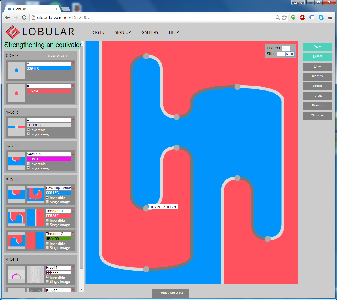
The main part of the screen shows a diagram, which in this case is 2-dimensional. It represents a composite 2-cell in a finitely-presented 2-category, with the blue and red regions representing objects, the lines representing 1-cells, and the vertices representing 2-cells. In fact, this 2d diagram is just an intermediate state of a 3d proof, through which we’re navigating with the ‘Slice’ controls in the top-right. The proof itself has been built up by composing the generators listed in the signature, down the left-hand side of the screen. (If you want to take a look at this proof yourself, you can go straight there; in the top-right, set ‘Project’ to 0, then increment the second ‘Slice’ counter to scroll through the proof.)

Globular has been developed so far in the Quantum Group in
the Oxford Computer Science department, by Krzysztof
Bar, Katherine Casey, Aleks Kissinger, Jamie Vicary and Caspar Wylie. We haven’t quite got around to it yet, but Globular will be open-source, and we’re really keen for people to get involved and help build the software—there’s a huge amount to do! If you want to help out, get in touch.

Mathematical foundations

Globular is based on the theory of finitely-presented semistrict n-categories; at the moment, it works up to the level of 3-categories, with an extension to 4-categories actively in development. (You can build cells of any dimension, but from 4-cells and up, some structures are missing.)

Definitions of n-category vary in how strict they are; a definition is semistrict when it’s as strict as possible, while still having the property that every weak n-category satisfies it, up to equivalence. Definitions of semistrict n-category are not unique: in dimension 3, Gray categories put all the weak structure in the interchangers, while Simpson snucategories put it all in the unitors. Globular implements the axioms of a Gray category, because this is the most appropriate for the graphical calculus: the interchangers can be seen graphically, as changes in height of the components of the diagram. By the theory of k-tuply monoidal n-categories, this also lets you build proofs in a monoidal category, or a braided monoidal category, or a monoidal 2-category.

The only things that Globular understands are -cells, for some value of . So if you want to build an n-category where an equation holds between n-cells, you have to do it by adding -cells and . If you then build some composite involving , you can apply the cell to obtain , and we interpret this as the equation . In a slogan, this is equality via rewriting. This is consistent with the basic premise of homotopy type theory: treat your proofs as first-order structures, which can in turn be reasoned about themselves.

Globular can also handle invertibility in a nice way. For a cell to be invertible, indicated by ticking a box in the signature, means that there also exists an invertible cell , and invertible cells and . This is a coinductive definition (see Mike Shulman’s nice post on this topic), since we’re defining the notion of invertibility in terms of itself in a higher dimension. This sort of a definition is great for proof assistants to work with, as it allows a lot of structure to be generated from a single compact definition.

How it works

For a lot more details, take a look at the nLab page. Everything that happens in Globular involves in interaction between the signature on the left-hand side, and the diagram in the main part of the screen. The signature stores the ‘library’ of cells you have available, and the diagram is a particular composite of cells that you have constructed.

To construct a new diagram, clear whatever is currently displayed by clicking the ‘Clear’ button on the right, or pressing ‘c’. Then start by clicking the icon of a n-cell in your signature, which will make a diagram consisting just of that cell. Clicking on the icons of other -generators for will display a list of ways the cell can be attached, and when you choose one of these ways, the attachment will be performed, growing your n-diagram. (If you’re starting with a blank workspace you will only have a single 0-cell available, so you won’t be able to do this yet!) Clicking an -cell displays a list of ways that your n-diagram can be rewritten, by identifying the source of as a subdiagram of . Selecting one of these ways will implement the rewrite, by ‘cutting out’ the chosen subdiagram of , and replacing it with the target of .

Another way to modify the diagram is to click directly on it. Clicking near the edge of the diagram performs an attachment, while clicking in the interior of the diagram performs a rewrite. If more than one attachment or rewrite is consistent with your click, a little menu will pop up for you to choose what you want to do. When you move your mouse pointer over the diagram, a little label pops up to show you what your cursor is hovering over, which is helpful when choosing where to click.

You can also click-and-drag on the diagram. This will attach or rewrite with an interchanger, or naturality for an interchanger, or invertibility for an interchanger, depending on where you have clicked and the direction of the drag. Clicking and dragging is designed to work as if you were really ‘touching’ the strings. So if you want to braid one strand over another, click the strand to ‘grab’ it, and ‘pull’ it to one side. If you want to pull a vertex through a braiding, click the vertex to ‘grab’ it, and ‘pull’ it up or down through its adjacent braiding. Of course, Globular will only carry out the command if the move you are attempting to make is actually valid in that location.

Example theorems

Here are four worked examples of nontrivial proofs in Globular:

• Frobenius implies associative: http://globular.science/1512.004. In a monoidal category, if multiplication and comultiplication morphisms are unital, counital and Frobenius, then they are associative and coassociative.

• Strengthening an equivalence: http://globular.science/1512.007. In a 2-category, an equivalence gives rise to an adjoint equivalence, satisfying the snake equations.

• Swallowtail comes for free: http://globular.science/1512.006. In a monoidal 2-category, a weakly-dual pair of objects gives rise to a strongly-dual pair, satisfying the swallowtail equations.

• Pentagon and triangle implies : http://globular.science/1512.002. In a monoidal 2-category, if a pseudomonoid object satisfies pentagon and triangle equations, then it satisfies .

We’ll focus on the second example project “Strengthening an equivalence” listed above, and see how it was constructed. This project investigates the factthat every equivalence in a 2-category gives rise to an adjoint equivalence. To start, we therefore need the basic data that exhibits an equivalence in a 2-category: two 0-cells and , and an invertible 1-cell , by the weak definition of ‘invertible’ discussed above. This gives us the following signature:

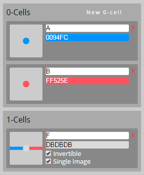
The 2-cells that witness invertibility of look like cups and caps in the graphical calculus, but they won’t satisfy the snake equations that define an adjoint equivalence. The idea of this proof is to define a new cap, built out of the invertible structure of , which does satisfy the snake equations with the existing cup.

By starting with a diagram consisting of alone, pressing ‘i’ to take the identity diagram, and clicking-and-dragging, we build the following 2-diagram, out of the invertible structure associated to :

This is our candidate for our redefined cup. Its source is the identity on , and its target is composed with . It looks a bit like the curved end of a hockey stick.

To store it for later use, we now click the ‘Theorem’ button. Writing for the 2-diagram we have constructed, this does two things. First, it creates a 2-cell generator that we call “New Cup”, whose source is , and whose target is . This is the redefined cup that we can use in future expressions. Second, it creates an invertible 3-cell generator that we call “New Cup Definition”, with source given by “New Cup”, and with target given by our hockey-stick diagram . This says what “New Cup” means in terms of our original structure. This adds the following cells to our signature:

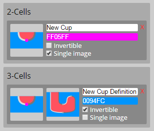
Because “New Cup Definition” is a 3-cell, by default we see two little icons: one for its source, and one for its target. See how its source is a little picture of “New Cup”, and its target is a little picture of the hockey stick, just as we defined it.

We’re now ready to prove one of the snake equations. We start by building the snake composite, using “New Cup” for the cup, and the invertible structure of for the cap:

Now have to prove that this equals the identity. Since equality is implemented by rewriting, we must construct a 3-diagram whose source is this snake composite, and whose target is the identity on . To start, we click the ‘Identity’ button to convert our diagram into an identity 3-diagram. The only apparent effect this has is to add a number scroller to the ‘Slice’ area of the controls in the top-right. At the moment we can set this to ‘0’ and ‘1’, representing the source and target of our identity 3-diagram respectively. We set it to ‘1’, because we want to compose things to the target.

We now build up our proof. First, we click on the pink vertex that represents “New Cup”. This will attach our 3-cell “New Cup Definition”, replacing “New Cup” with our hockey-stick picture. By clicking-and-dragging on the diagram, we obtain the following sequence
of pictures:

           

             
 

Pictures 3 to 10 were created by attaching interchangers, and pictures 11 to 15 were created by attaching higher structure generated by the invertibility of . In all cases, this structure was attached just by clicking-and-dragging on the appropriate vertices of the diagram. We’ve turned the snake into the identity, so we’ve finished our proof, which required 14 3-cells. By using the ‘Slice’ control in the top-right, we can navigate through the 15 slices that make up our proof, and review what we just did. Even better, turning the ‘Project’ control to the value ‘1’ tells Globular to project out the lowest dimension. This means that our entire 3-diagram proof can be viewed as a single 2-dimensional diagram, as follows:

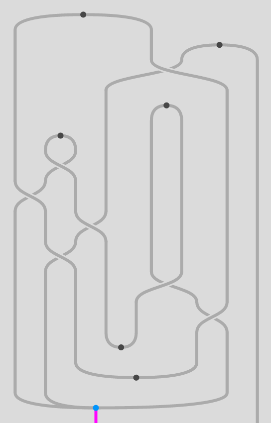
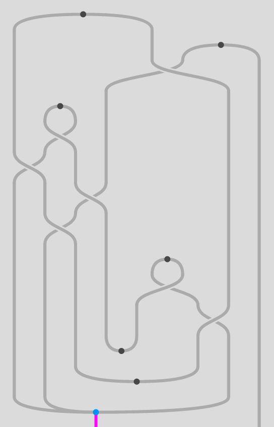
This is just like the Morse singularity graphics used by topologists to study the structure of higher-dimensional manifolds. In this picture, the vertices are 3-cells, the lines are 2-cells, and the regions are 1-cells (in fact, every region is the 1-cell .) By moving your mouse pointer over the different parts of the diagram, you can see what the different components are. Interchangers are represented in this projection by braidings.

Now we can do something cool: we can modify our proof, by clicking-and-dragging on the Morse projection. For example, just to the right of centre, there is a crossing, out of which emerge two long vertical lines that travel up a long way before annihilating with one another. Our proof would be much simpler if these two lines just annihilated with each other right after the interchanger. So, we click the vertex at the top of the lines, and drag it down repeatedly, until it gets to where we want it:

We’ve simplified our proof. By clicking-and-dragging some more, you can change the proof in lots of different ways, although you probably won’t get it much simpler than this. Putting the ‘Project’ control back to ‘0’, and navigating through the stages of the proof with the ‘Slice’ control as we were doing before, we can see that our proof has indeed been modified.

This project has been in development for about 18 months, so it feels great to finally launch. We hope the whole community will get clicking-and-dragging, and let us know how easy it is to use, and what other features would be useful. There are certain to still be bugs, so let us know about them too, and we’ll get right on them.