Here’s a cute connection between topological entropy, braids, and the golden ratio. I learned about it in this paper:
• Jean-Luc Thiffeault and Matthew D. Finn, Topology, braids, and mixing in fluids.
Topological entropy
I’ve talked a lot about entropy on this blog, but not much about topological entropy. This is a way to define the entropy of a continuous map 

How can we make this precise? First, cover 


Of course the answer depends on 

And of course the answer also depends on our choice of open cover

Believe it or not, this is often finite! Even though the log of the number of symbol strings we get will be larger when we use a cover with lots of small sets, when we divide by 
Braids
Any braid gives a bunch of maps from the disc to itself. So, we define the entropy of a braid to be the minimum—or more precisely, the infimum—of the topological entropies of these maps.
How does a braid give a bunch of maps from the disc to itself? Imagine the disc as made of very flexible rubber. Grab it at some finite set of points and then move these points around in the pattern traced out by the braid. When you’re done you get a map from the disc to itself. The map you get is not unique, since the rubber is wiggly and you could have moved the points around in slightly different ways. So, you get a bunch of maps.
I’m being sort of lazy in giving precise details here, since the idea seems so intuitively obvious. But that could be because I’ve spent a lot of time thinking about braids, the braid group, and their relation to maps from the disc to itself!
This picture by Thiffeault and Finn may help explain the idea:

As we keep move points around each other, we keep building up more complicated braids with 4 strands, and keep getting more complicated maps from the disc to itself. In fact, these maps are often chaotic! More precisely: they often have positive entropy.
In this other picture the vertical axis represents time, and we more clearly see the braid traced out as our 4 points move around:

Each horizontal slice depicts a map from the disc (or square: this is topology!) to itself, but we only see their effect on a little rectangle drawn in black.
The golden ratio
Okay, now for the punchline!
Puzzle 1. Which braid with 3 strands has the highest entropy per generator? What is its entropy per generator?
I should explain: any braid with 3 strands can be written as a product of generators 


For any braid we can write it as a product of 
Now for the answer to the puzzle!
Answer 1. A 3-strand braid maximizing the entropy per generator is 

In other words, the entropy of this braid is

All this works regardless of which base we use for our logarithms. But if we use base e, which seems pretty natural, the maximum possible entropy per generator is

Or if you prefer base 2, then each time you stir around a point in the disc with this braid, you’re creating

bits of unknown information.
This fact was proved here:
• D. D’Alessandro, M. Dahleh and I Mezíc, Control of mixing in fluid flow: A maximum entropy approach, IEEE Transactions on Automatic Control 44 (1999), 1852–1863.
So, people call this braid 
What does it all mean? Well, the 3-strand braid group is called 
• John Baez, This Week’s Finds in Mathematical Physics (Week 233).
You’ll see there that
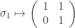

These matrices are shears, which is connected to how the braids
I guess this must be part of the story too:
Puzzle 2. Is it true that when we multiply
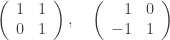
or their inverses:

the magnitude of the largest eigenvalue of the resulting product can never exceed the
There’s also a strong connection between braid groups, certain quasiparticles in the plane called Fibonacci anyons, and the golden ratio. But I don’t see the relation between these things and topological entropy! So, there is a mystery here—at least for me.
For more, see:
• Matthew D. Finn and Jean-Luc Thiffeault, Topological optimisation of rod-stirring devices, SIAM Review 53 (2011), 723—743.
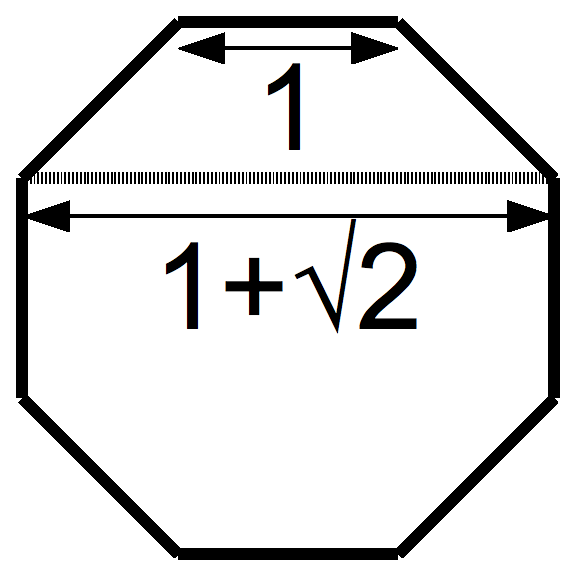
Abstract. There are many industrial situations where rods are used to stir a fluid, or where rods repeatedly stretch a material such as bread dough or taffy. The goal in these applications is to stretch either material lines (in a fluid) or the material itself (for dough or taffy) as rapidly as possible. The growth rate of material lines is conveniently given by the topological entropy of the rod motion. We discuss the problem of optimising such rod devices from a topological viewpoint. We express rod motions in terms of generators of the braid group, and assign a cost based on the minimum number of generators needed to write the braid. We show that for one cost function—the topological entropy per generator—the optimal growth rate is the logarithm of the golden ratio. For a more realistic cost function,involving the topological entropy per operation where rods are allowed to move together, the optimal growth rate is the logarithm of the silver ratio,
We show how to construct devices that realise this optimal growth, which we call silver mixers.
Here is the silver ratio:
But now for some reason I feel it’s time to stop!


Non-specialist comment: Is there an application to energy-efficient mixing here? That is can we modify the gearing and mechanics of typical blenders to blend things more completely more quickly, thereby using less power….more “green”?
I tend to think of this result as more about beautiful pure math than anything practical, but there are related papers that focus on the practical issue of efficient mixing. Since real-world mixing is about 3-dimensional fluids, it’s a lot more complicated. It’s very interesting, but I don’t know much about it.
On the lighter side, see:
• Jean-Luc Thiffeault, A mathematical history of taffy pullers.
This paper has 56 pictures and is definitely worth a look! I never knew the mathematics of taffy was so interesting.
I love the apparent real world usability of this!
Don’t get me wrong, I also love pure maths (even if my understanding is very limited as this point), but it’s a rather surprising, unexpected use case, so that’s lovely in its own right.
Also, watching that taffy puller is mesmerizing.
Solution to Puzzle 2:
If you apply any of the four matrices to a vector , you obtain a vector
  such that
and
Hence if we apply any sequence of matrices, repeated
  times, these two invariants are bounded by the
  th entry of a Fibonacci-like sequence. So they are bounded by a constant times the
  th power of the golden ratio. If the starting vector is an eigenvector, both invariants grow like the
  th power of the eigenvalue, so the eigenvalue is at most the
  th power of the golden ratio.
Yes – nice!
Coming very late to this but just came across this page while really enjoying looking through the rest of the blog. Will in the comment above has already answered puzzle 2 – Thiffeault and I produced some fairly tight bounds on that eigenvalue (actually the Lyapunov exponent, but essentially the same thing) here: https://link.springer.com/article/10.1007/s00332-018-9497-3 . The argument is knowing that the vectors stay in an invariant cone in tangent space, and knowing the probability distribution of repeated occurrences of each matrix.
Thanks, I’ll check it out sometime!