It sounds like jargon from a bad episode of Star Trek. But it’s a real thing. It’s a monstrous object that lives in the plane, but is impossible to draw.
Do you want to see how snake-like it is? Okay, but beware… this video clip is a warning:
This snake-like monster is also called the ‘pseudo-arc’. It’s the limit of a sequence of curves that get more and more wiggly. Here are the 5th and 6th curves in the sequence:

Here are the 8th and 10th:

But what happens if you try to draw the pseudo-arc itself, the limit of all these curves? It turns out to be infinitely wiggly—so wiggly that any picture of it is useless.
In fact Wayne Lewis and Piotr Minic wrote a paper about this, called Drawing the pseudo-arc. That’s where I got these pictures. The paper also shows stage 200, and it’s a big fat ugly black blob!

But the pseudo-arc is beautiful if you see through the pictures to the concepts, because it’s a universal snake-like continuum. Let me explain. This takes some math.
The nicest metric spaces are compact metric spaces, and each of these can be written as the union of connected components… so there’s a long history of interest in compact connected metric spaces. Except for the empty set, which probably doesn’t deserve to be called connected, these spaces are called continua.
Like all point-set topology, the study of continua is considered a bit old-fashioned, because people have been working on it for so long, and it’s hard to get good new results. But on the bright side, what this means is that many great mathematicians have contributed to it, and there are lots of nice theorems. You can learn about it here:
• W. T. Ingraham, A brief historical view of continuum theory,
Topology and its Applications 153 (2006), 1530–1539.
• Sam B. Nadler, Jr, Continuum Theory: An Introduction, Marcel Dekker, New York, 1992.
Now, if we’re doing topology, we should really talk not about metric spaces but about metrizable spaces: that is, topological spaces where the topology comes from some metric, which is not necessarily unique. This nuance is a way of clarifying that we don’t really care about the metric, just the topology.
So, we define a continuum to be a nonempty compact connected metrizable space. When I think of this I think of a curve, or a ball, or a sphere. Or maybe something bigger like the Hilbert cube: the countably infinite product of closed intervals. Or maybe something full of holes, like the Sierpinski carpet:
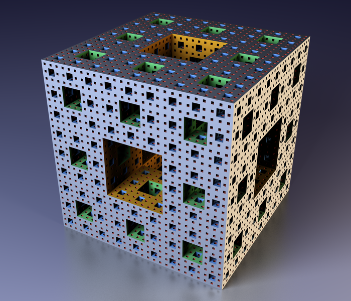
or the Menger sponge:
Or maybe something weird like a solenoid:
Very roughly, a continuum is ‘snake-like’ if it’s long and skinny and doesn’t loop around. But the precise definition is a bit harder:
We say that an open cover 𝒰 of a space X refines an open cover 𝒱 if each element of 𝒰 is contained in an element of 𝒱. We call a continuum X snake-like if each open cover of X can be refined by an open cover U1, …, Un such that for any i, j the intersection of Ui and Uj is nonempty iff i and j are right next to each other.
Such a cover is called a chain, so a snake-like continuum is also called chainable. But ‘snake-like’ is so much cooler: we should take advantage of any opportunity to bring snakes into mathematics!
The simplest snake-like continuum is the closed unit interval [0,1]. It’s hard to think of others. But here’s what Mioduszewski proved in 1962: the pseudo-arc is a universal snake-like continuum. That is: it’s a snake-like continuum, and it has continuous map onto every snake-like continuum!
This is a way of saying that the pseudo-arc is the most complicated snake-like continuum possible. A bit more precisely: it bends back on itself as much as possible while still going somewhere! You can see this from the pictures above, or from the construction on Wikipedia:
• Wikipedia, Pseudo-arc.
I like the idea that there’s a subset of the plane with this simple ‘universal’ property, which however is so complicated that it’s impossible to draw.
Here’s the paper where these pictures came from:
• Wayne Lewis and Piotr Minic, Drawing the pseudo-arc, Houston J. Math. 36 (2010), 905–934.
The pseudo-arc has other amazing properties. For example, it’s ‘indecomposable’. A nonempty connected closed subset of a continuum is a continuum in its own right, called a subcontinuum, and we say a continuum is indecomposable if it is not the union of two proper subcontinua.
It takes a while to get used to this idea, since all the examples of continua that I’ve listed so far are decomposable except for the pseudo-arc and the solenoid!
Of course a single point is an indecomposable continuum, but that example is so boring that people sometimes exclude it. The first interesting example was discovered by Brouwer in 1910. It’s the intersection of an infinite sequence of sets like this:

It’s called the Brouwer–Janiszewski–Knaster continuum or buckethandle. Like the solenoid, it shows up as an attractor in some chaotic dynamical systems.
It’s easy to imagine how if you write the buckethandle as the union of two closed proper subsets, at least one will be disconnected. And note: you don’t even need these subsets to be disjoint! So, it’s an indecomposable continuum.
But once you get used to indecomposable continua, you’re ready for the next level of weirdness. An even more dramatic thing is a hereditarily indecomposable continuum: one for which each subcontinuum is also indecomposable.
Apart from a single point, the pseudo-arc is the unique hereditarily indecomposable snake-like continuum! I believe this was first proved here:
• R. H. Bing, Concerning hereditarily indecomposable continua, Pacific J. Math. 1 (1951), 43–51.
Finally, here’s one more amazing fact about the pseudo-arc. To explain it, I need a bunch more nice math:
Every continuum arises as a closed subset of the Hilbert cube. There’s an obvious way to define the distance between two closed subsets of a compact metric space, called the Hausdorff distance—if you don’t know about this already, it’s fun to reinvent it yourself. The set of all closed subsets of a compact metric space thus forms a metric space in its own right—and by the way, the Blaschke selection theorem says this metric space is again compact!
Anyway, this stuff means that there’s a metric space whose points are all subcontinua of the Hilbert cube, and we don’t miss out on any continua by looking at these. So we can call this the space of all continua.
Now for the amazing fact: pseudo-arcs are dense in the space of all continua!
I don’t know who proved this. It’s mentioned here:
• Trevor L. Irwin and Salawomir Solecki, Projective Fraïssé limits and the pseudo-arc.
but they refer to this paper as a good source for such facts:
• Wayne Lews, The pseudo-arc, Bol. Soc. Mat. Mexicana (3) 5 (1999), 25–77.
Abstract. The pseudo-arc is the simplest nondegenerate hereditarily indecomposable continuum. It is, however, also the most important, being homogeneous, having several characterizations, and having a variety of useful mapping properties. The pseudo-arc has appeared in many areas of continuum theory, as well as in several topics in geometric topology, and is beginning to make its appearance in dynamical systems. In this monograph, we give a survey of basic results and examples involving the pseudo-arc. A more complete treatment will be given in a book dedicated to this topic, currently under preparation by this author. We omit formal proofs from this presentation, but do try to give indications of some basic arguments and construction techniques. Our presentation covers the following major topics: 1. Construction 2. Homogeneity 3. Characterizations 4. Mapping properties 5. Hyperspaces 6. Homeomorphism groups 7. Continuous decompositions 8. Dynamics.
It may seem surprising that one can write a whole book about the pseudo-arc… but if you like continua, it’s a fundamental structure just like spheres and cubes!


I’ll just say: I don’t see that as a bucket handle – and leave it at that!
In an email, Wayne Lewis also pointed this out:
For those not in the know, a Gδ set is a countable intersection of open sets. A dense set is a countable intersection of open dense sets, so its complement is meager.
So, if one ever spends any length of time goofing around at the intersection of number theory and fractals, you’ll see lots and lots of figures resembling the pseudo-arc. (and its brand new news to me to find out they’re called pseudo-arcs). Whenever one encounters one of these things, there’s an interesting game one can play: draw a horizontal line through the figure, and count how many intersections it has. For each height of the horizontal line, one gets a different count, and making a graph of that vs. height, one typically discovers some fractal measure.
I call it a “measure”, well, because its integrable. Certainly, the count is always positive, and, for any fixed you can find a way to normalize it so the integral is 1.0.
As you take the limit of you’ll typically find peaks that grow without bound, valleys that stay small, and a general self-similar behavior. The integrals will have a “devil’s staircase” type behavior. The most famous example is the distribution of the Farey numbers, which turns out to be exactly equal to the “derivative” of the Minkowski question-mark function. But once you get going, you find them just absolutely everywhere, all maddeningly similar and yet all different, and working out a way of characterizing them seems to become the holy grail.
I’m tempted to run off and attempt this process on the pseudo-arc. Hmm.
Looking at the Lewis and Minic paper, one sees the words “Fibonacci-like sequence”, and, whenever one sees those words, (or the words “the golden ratio”), its inevitable that the authors are looking at a special case of the modular group, viz of the Mobius fractions (ax+b)/(cx+d) with a,b,c,d integers and ad-bc=1. The Fibonacci sequence is the special case of a=1, b=0 c=2 d=1 or something like that. I forget exactly what. The modular group has an extremely rich theory connecting continued fractions, elliptic curves, Riemann zeta zeros and more. Things like the crookedness sequence are rampant (you can build one for any a,b,c,d of the above form) and the n-crooked maps arise naturally in all kinds of different settings.
For example: Definition 3.8 on page 10 of the Lewis and Minic paper, the simple simple n-crooked map is defined using
This is easily generalized to
although you also have to use the appropriate generalized cr[] function. In this form its recognizable as a partial convergent for a continued fraction; it was famously studied by Kuzmin and by Ramanjuan; the former developing it into a theory of continued fractions and the later into a proto-theory of modular forms. It’s sort of an infinite maze of interconnecting, interesting things; for example, a hop-skip & jump away is monstrous moonshine; while in another direction there are the Teichmüller spaces and moduli spaces.
Cool stuff, Linas. Can you get a pseudo-arc as the result of some specific number-theory-related problem? That would be really interesting.
One can argue that it will be unsurprising if you succeed, given that pseudo-arcs are “common” (for example, dense in the space of all continua). However, even unsurprising things can be interesting to actually know.
In their paper Drawing the pseudo-arc, Lewis and Minic suggest that it should be possible to obtain the pseudo-arc as the attractor of some chaotic dynamical system, and they give some hints for how to proceed… but they do not exhibit such a system. So, this is another place one should look for a pseudo-arc.
Hmm. Well, the answer required much closer reading and thinking, and the answer is “no”. First, let me explain why I suggested earlier that the answer is “yes”. The construction, the accompanying images all look like fairly generic recursive fractal constructions, and lord-knows I’ve stared at too many of those. I searched for something similar that I might have had lying around, and created a folder of detritus from my notebooks, which are all vaguely snake-like images that fail to satisfy the definition of the pseudo-arc. This hopefully explains my initial “oh, that” knee-jerk reaction (that, and it was very late Sunday night). It doesn’t help that the solenoid and the buckethandle are “ordinary” period-doubling Cantor-set style constructions. There’s countless numbers of those.
The reality is that the definition of the pseudo-arc does not allow some ordinary fractal, period-doubling-style construction, even though the diagrams in Lewis and Minic superficially suggest that it might be. All “ordinary” fractals are set either in Cantor space or in Baire space
  and continued fractions provide a way of bouncing from one to the other. Both of these spaces are (infinite) Cartesian products of discrete spaces, and the mappings from this product topology to the natural topology on Euclidean space is what makes fractals fractal-ish. These two spaces are shift spaces, which essentially explains all of the self-similarity properties of fractals. There are more kinds fractals than just this, but this takes care of the vast majority of the commonly seen ones — all of the “period-doubling” kind.
The pseudo-arc is not of this kind. I’m having trouble figuring out what kind it is. The crux of the matter is how one labels the “points” in the pseudo-arc. For example, in ordinary period-doubling, Cantor-set-style fractal curves or dusts, its enough to specify an infinite string of left-right moves, or binary digits to specify a “point”; a finite string of these specifies the “general area” that one is zooming into. For the pseudo-arc, it seems like one would have to specify an infinite sequence of finite sequences of choices from the set {bottom,slash,top} of the Z-shape of a zig-zag. At each stage, the sequence has to be at least twice-the-Pell-number longer. Or something like that. It’s unaccustomed territory for me, and I have not actually seen anything like that before.
Actually there has been some progress on getting the pseudo-arc to show up as an attractor. You can see it on page 476 of Mayer and Overstegen’s chapter ‘Continuum Theory’ in the 1992 book Recent Progress in General Topology edited by M. Husek and J. van Mill.
Well, the 1980’s was the heyday of chaotic attractors. Some of what I was mentioning only emerged in the 90’s and 2000’s after the dust settled a bit. It seems “intuitively clear” that the Henon or Ueda attractors resemble the buckethandle or Smale horseshoes, which can be arrived at slightly more rigorously by considering the stable and unstable manifolds of the attractor. And when one has that, namely the horocycles and the foliations and the Hopf-fibration-style decompositions into the stable and unstable manifolds, then one can understand the dynamics as iterations of block-diagonal matrices, (aka “symbolic dynamics”, “sofic systems”, “measure-preserving dynamical systems” etc.) and whenever you iterate a block-diagonal matrix, you’re dealing with a shift space, and whenever you’ve got a shift space, your dealing with the product topology on some (that is, the countable product of some discrete set
  ), and soon as you have the product topology, you’ve got “ordinary” fractals. So, in that sense, the Henon map is “ordinary”. (Yes, sure, there are subtle details, e.g. the homoclinic orbits, and other difficulties I’m glossing over. But the general picture stands.)
The point is that the pseudo-arc is not of this ordinary type, its much worse; it kind-of behaves badly everywhere. The crooked folding is everywhere-dense. This is in sharp contrast to the buckethandle, the Smale horseshoe, the Baker’s map, which squeeze in one dimension and stretch in another and resemble squashed pancakes – they’re essentially flat-everywhere, except at the folds. Its also in contrast to e.g. the “blancmange curve”, which is everywhere-crooked but fails to satisfy the definition of the pseudo-arc, because the crookedy-parts don’t fold back on themselves “far enough”, they don’t get to within epsilon of the starting point.
The clearest example of the jargon I’m juggling is in the Anosov diffeomorphism article, the bulk of which I wrote 12 years ago, it seems. Its a special case of an Axiom A system. The Henon map is not Axiom A, its kind of non-uniform in how its hyperbolic, but it still “pancakes”, it’s not “wild everywhere” the way the pseudo-arc is.
I apologize for posting so much, I suspect its kind of annoying, so I will try to stay quiet now.
It’s not annoying! These days it’s usually too quiet on this blog—I wish there were more comments. It’s my fault, because I’m so busy with my grad students and other things that I no longer talk about my ideas here as much as I used to.
I used to know the definitions of phrases like ‘axiom A’, ‘pseudo-Anosov’ etc., back when I was regularly reading Abraham and Marsden’s Foundations of Mechanics. But I never really got deep into the study of these things, so my knowledge was superficial and has by now faded.
I don’t have a great desire to study dynamical systems, chaos and the like—it’s a wonderful subject, but I don’t have something I’m trying to do with it, so I don’t feel a compulsion to master it. The last couple weeks I’ve been trying to understand [continua](https://en.wikipedia.org/wiki/Continuum_(topology) a little bit better. This little burst of enthusiasm reminds me of how I spent some time trying to learn the structure theory of 1) commutative monoids and 2) locally compact Hausdorff abelian groups. These structures, like continua, are too complicated to fully classify, but there are structure theorems giving partial classifications, and it was fun to spend some time delving in to them. In those two cases, however, I was working on a project where I really needed to learn the stuff.
In the process, I’m gathering up pretty pictures for a planned reboot of Visual Insight. (And indeed, I can imagine wanting to study dynamical systems and fractals just as a way to gather more pretty pictures for that blog!)
Dynamical systems can be fun because they can touch on so many topics. So: in “symbolic dynamics”, do the symbol sequences form a language, and what’s that language? This leads to finite state machines, which leads to acts, groupoids, etc. or to geometric state machines (quantum state machines when the homogenous space comes from a unitary group). Languages also show in computing, in model theory, in logic, should you go that far.
Some of the simpler chaotic systems are geodesics on hyperbolic spaces, such as on elliptic curves, or on Riemann surfaces, both which lead into number theory. But notions of modular forms in a general setting eventually lead into the big bulk of differential topology. Along the way, you get to ask about spectra and operators.
Dynamical systems in a narrow sense happen on symplectic manifolds, which is what Abraham & Marsden explain. One can thence journey to affine geometry on fibre bundles. Or to Riemannian geometry which seems prettiest when there’s a spin structure. Which leads to Clifford algebras and tensor algebras and Hopf algebras and those pesky affine Lie algebras. Once they’ve seen the spin group and the string group, how you gonna keep them down on the farm? So dynamical systems can be a kind of “come for the pretty pictures, stay for the math”. Although this line of reasoning does stab chaos theory in the back, leaving it dead on the road.
The most intriguing part of dynamical systems, to me, is the transfer operator. This operator replaces point dynamics (where did this trajectory/geodesic go?) by the dynamics of smooth distributions (how does the ensemble/bulk evolve?). The most shocking thing that it does is to take systems that seem time-reversible (when viewed as individual trajectories) and make them time-irreversible (when viewed as a bulk). Eigenvalues aren’t unitary, they’re less than one. Its the device that takes you from ergodic theory and into mixing, so when you ask “where did the arrow of time come from?”, this is the correct place to look, the correct device to apply.
This has lead me on several occasions to blurt out to you some imprudent musings which you aren’t ever receptive to – it’s OK, I know they sound kooky. I just have this gut sense that taking an ensemble, transfer-operator-type viewpoint/approach to the differential eqns of ye-olde canonical quantum has the potential to .. oh never mind. Life is short; I won’t have the time to ever finish that thought. Its like the candy at the far end of the candy store, too many distractions between here and there.
I can offer up some of those. They’re devoid of difficult math, and offer no insight into any traditional branches of math, but they’re pretty (to me). http://linas.org/art-gallery/gpf/gpf.html and also this: http://linas.org/art-gallery/arithmexpic/arithmexpic.html
Linas wrote:
All math is connected… but I probably know about ten times more about any one of these other topics than I do about dynamical systems, so invoking them mainly reminds me that I’m more interested in all these other subjects than dynamical systems!
I could get interested in dynamical systems… but only if I had some project or hobby that would pull me in.
For example, one thing I’d like to understand is why in celestial resonance sometimes seems to stabilize orbits and sometimes seems to destabilize them. For example, the moons of Jupiter seem to ‘enjoy’ being in resonance:
but the rings of Saturn have gaps at orbits that are in resonance with the moons:
As you probably know, this subject is sometimes called Koopmanism. Prigogine has talked a lot about the ’emergent irreversibility’ that arises from this viewpoint. I guess a good intro is here:
• B. Misra, I. Prigogine and M. Courbage, From deterministic dynamics to probabilistic descriptions, Physica A: Statistical Mechanics and its Applications 98 (1979), 1–26.
This is another aspect of dynamical systems I could get interested in. I’m always interested in the ‘arrow of time’, and there seems to be some nice math here.
Disclaimer: I’ve never done astrodynamics! The simplest model I know of for phase-locking is the kicked rotor and the circle map. The laboratory-bench device consists of two disks; one is free to spin, the other is attached to a motor. A weak, stretchy spring connects to a point on each rim. You turn on the motor, and the freely-spinning disk will turn also, pulled by the spring. The speed of the freely-spinning disk will quickly lock into some integer ratio of the motor; the dominant ones being 1:1 but also 2:1, 1:4 will be strong phase-locking regions. In principle, it can phase lock to any integer ratio p:q, although most of these are very weak and hard to lock onto. In electronics, phase-locked loops (PLL’s) use this principle to lock onto a radio signal; they’re very widespread.
The mathematical model for this is the “circle map”, the iterated equation The value of
  can be thought of as the angle of the spinning disk. The constant value of
  can be thought of as the frequency of the driving motor. The small constant
  is supposed to be the weak coupling of the spring. Basically, if the freely-spinning disk races ahead, the K pulls it back. If it lags, it gets pushed forward.
There are two free parameters: the speed of the motor, the strength of the spring. What happens? Either it phase locks promptly, or its its in a region where it has trouble locking on, and bounces chaotically. The phase-locked regions are called Arnold tongues, the wikipedia article has explanations and pretty pictures (made by me). There are more here – a tall one, a close-up and a different closeup. They’re pretty.
The orbital dynamics problem would be solved by picking a set of orbital coordinates for the moons, discover that the forces between them resemble the circle map (replacing the sine by some other periodic function, as needed), and then concluding “ah hah!”. I assume this just all works out with maybe some interesting hiccups along the way.
The clearing of the dust lanes starts the same way, except that now one realizes one is also dealing with an Anosov flow. If you placed two pieces of dust near each other in a dust-free lane, two things happen. The phase-locking forces would probably push them closer to one-another in the angular direction, but pull them apart in the radial direction. This is characteristic of Anasov flows: in some directions, trajectories (geodesics) converge; in other (orthogonal) directions, they diverge. The expanding, diverging geodesic flows clear the dust-free lanes.
Traditionally, these would be called “tidal forces”, appearing in the stress tensor, but I find that name unintuitive for this particular setting: Its really the geodesic flow, the integral curves, the visual shape of tangent manifolds that is visualizable, that can be captured in a motion-picture. Telling someone “oh its just tides” is utterly unintuitive.
BTW, such flows also have some “neutral” directions, orthogonal to the stretch and compress directions. Here, this would be the direction orthogonal to the orbital plane — there are no forces in that direction.
Motion in the dusty lanes is chaotic and mixing (in the formal sense of mixing), so if you could drop a bag of brightly colored glitter into one of the dust lanes, you’d find that it spread all over the place in short order.
So the above is the “physical”, “intuitive” explanation, and again, its pure speculation on my part, but I believe its correct. Some remarks: first about topology. The Arnold tongues map a set of measure zero (the rationals) into a set of finite measure (the tongues, one distinct, unique tongue per rational). How does that work? Seems magical to me. I really don’t get it. Topology is weird.
The appearance of lanes suggests that there is some operator having some spectrum. What’s that operator? How is it related to the transfer operator (and what is the transfer operator for these problems, anyway?). (The transfer operator is what tells you about the bulk motion of dust). I’ve never, ever seen even a hint of a discussion of this, anywhere. For me, personally, it would be a good excuse to study index theorems, although they might have little relation to the problem. Developing an operator-theoretic understanding of this phenomena is what would interest me.
The Koopman operator is the one-sided inverse to the transfer operator
  so that
  but
but  . The simplest time-irreversability discussion I know of is Fully Chaotic Maps and Broken Time Symmetry | Dean Driebe | Springer There’s actually a much simpler way of presenting his material, but, whatever. The transfer/koopman operators show up in special functions, where they relate multiplicative functions from number theory to the multiplication theorem for the gamma function, polylogarithm, Bernoulli polynomials etc. The special functions are essentially the eigenfunctions of the koopman/transfer operators that correspond to the multiplicative functions.
I once saw a “koopmanistic” lecture of the pre-quantization (expansion to first order in ) of billiards-in-a-box (ideal gas) and it was excellent and fascinating and I’ve been killing myself to find it again. The wave functions were fractals! They destructively interfere when all the billiards are on one side of the box! For things like the transfer operator of the Bernoulli map, one can “trivially” exhibit fractal eigenfunctions, so not a total surprise, but an ideal gas is a step up in sophistication.
The Moyal product of pre-quantization is a special case of the star product on universal enveloping algebras. This suggests that universal enveloping algebras have, um, fractal eigenfunctions in them, in general. You will just hate me for saying this, but, it seems that possibly, in general, operators with discrete spectra that have smooth eigenfunctions for those spectral points, also have fractal eigenfunctions (viz nowhere differentiable) with a continuous spectrum. I can show you special cases, but they’re hard to construct and hard to characterize and generalize. Connecting those dots would be interesting, but again, life is short.
A fascinating distinction for fractal-like objects! Tell me, are dragon curves more like the period-doubling examples, or more like the everywhere-difficult examples?
I dabbled a bit in the intersection of number theory
and fractals. Something i saw was a connection between
the Calkin-Wilf sequence
https://en.wikipedia.org/wiki/Calkin-Wilf_tree
and the Sharkovskii order
https://en.wikipedia.org/wiki/Sharkovskii%27s_theorem
on the positive integers. The Calkin-Wilf sequence is
a bijection from the positive integers to the positive
rationals. The recurrence relation,
is a concise expression for generating the sequence ). The Sharkovskii order is based on a
(
collection of sequences of positive integers which help
account for the structure of the standard period
doubling diagram.
For positive integers j,k the partially open rectangles
help describe symmetries in the graph of
 ).
).
(for k=1 set
Let be the intersection of the graph of
 with
with  .
.  is
is
empty if j<k. The function
is a bijection from to
to
 . Each
  is
is
invariant under the “reflections”
but an with more than 1 point is only
invariant under the “rotation”
The center of symmetry of is
is
 . This point is
 if and only if j=k. It is the only
 . For
. For  the
the doubles as we
in
point in
number of points in
increment j while keeping k fixed.
This is not very surprising since the intervals
 double in length as we
 , contains the image of the sequence
increment j. However the top row of rectangles,
3, 5, 7, 9, 11, …
The row of rectangles below it contains the image of
the sequence
In general, for a fixed k the rectangles,
$\latex R_{j,k}$, contain the image of the sequence
This sequence of sequences defines the Sharkovskii
 . These point sort of form the
order on the positive integers aside from the powers of
2. The powers of 2 are mapped by q to the bottom left
vertex on the boundary of the rectangles
bottom of the graph of q(N). And the powers of 2 form
the final sequence in the Sharkovskii order.
Thanks for the connection of Sharkovskii order to period doubling.
Here is some applied math/physics–
From working on the ENSO model, it’s clear that a period doubling exists in the ENSO time series. Many climate researchers believe that this time-series is chaotic, almost to the point of being snake-like. Yet, put together a period-doubling (i.e. annual to biennial) amplification on top of the highly precise cyclic lunar forcing and this may deconvolute the mess. I will present these results next week at the AGU meeting. This is a fit one can achieve without too much trouble:

It looks like the two time series match fairly well and so perhaps there will be no El Nino until 2019.
Over on G+, Matt McIrvin pointed out that the ‘crookedness numbers’ in this paper:
• Wayne Lewis and Piotr Minic, Drawing the pseudo-arc, Houston J. Math. 36 (2010), 905–934.
obeying
are usually called Pell numbers, and have been well-studied.
I asked Wayne Lewis if he ever wrote his promised book on the pseudo-arc and he said no, it was too hard.
Here is a nice article on the connection between the modular group (and thus, implicitly, number theory) and chaotic dynamical systems:
• Erwan Lanneau, Tell me a pseudo-Anosov, Newsletter of the European Mathematical Society 106 (December 2017), 11–16.
Only just saw this article now (which I think means I only glanced at it before, but now I’m more drawn in). I forget now just how I bumped into pseudo-arcs in the first place, but some of the intriguing recent thinking has to do with model theory and Fraïssé limts in a dual form. David Corfield seems to have picked up on this thread years and years ago: https://golem.ph.utexas.edu/category/2009/11/fraisse_limits.html
I guess this paper I mentioned is connected to that:
• Trevor L. Irwin and Salawomir Solecki, Projective Fraïssé limits and the pseudo-arc.