Open Systems in Classical Mechanics

I think we need a ‘compositional’ approach to classical mechanics. A classical system is typically built from parts, and we describe the whole system by describing its parts and then saying how they are put together. But this aspect of classical mechanics is typically left informal. You learn how it works in a physics class by doing lots of homework problems, but the rules are never completely spelled out, which is one reason physics is hard.

I want an approach that makes the compositionality of classical mechanics formal: a category (or categories) where the morphisms are open classical systems—that is, classical systems with the ability to interact with the outside world—and composing these morphisms describes putting together open systems to form larger open systems.

There are actually two main approaches to classical mechanics: the Lagrangian approach, which describes the state of a system in terms of position and velocity, and the Hamiltonian approach, which describes the state of a system in terms of position and momentum. There’s a way to go from the first approach to the second, called the Legendre transformation. So we should have a least two categories, one for Lagrangian open systems and one for Hamiltonian open systems, and a functor from the first to the second.

That’s what this paper provides:

• John C. Baez, David Weisbart and Adam Yassine, Open systems in classical mechanics.

The basic idea is by not new—but there are some twists! I like treating open systems as cospans with extra structure. But in this case it makes more sense to use spans, since the space of states of a classical system maps to the space of states of any subsystem. We’ll compose these spans using pullbacks.

For example, suppose you have a spring with rocks at both ends:

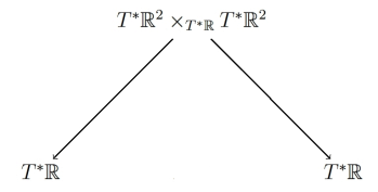
If it’s in 1-dimensional space, and we only care about the position and momentum of the two rocks (not vibrations of the spring), we can say the phase space of this system is the cotangent bundle

But this system has some interesting subsystems: the rocks at the ends! So we get a span. We could draw it like this:

but what I really mean is that we have a span of phase spaces:

Here the left-hand arrow maps the state of the whole system to the state of the left-hand rock, and the right-hand arrow maps the state of the whole system to the state of the right-hand rock. These maps are smooth maps between manifolds, but they’re better than that! They are Poisson maps between symplectic manifolds: that’s where the physics comes in. They’re also surjective.

Now suppose we have two such open systems. We can compose them, or ‘glue them together’, by identifying the right-hand rock of one with the left-hand rock of the other. We can draw this as follows:

Now we have a big three-rock system on top, whose states map to states of our original two-rock systems, and then down to states of the individual rocks. This picture really stands for the following commutative diagram:

Here the phase space of the big three-rock system on top is obtained as a pullback: that’s how we formalize the process of gluing together two open systems! We can then discard some information and get a span:

Bravo! We’ve managed to build a more complicated open system by gluing together two simpler ones! Or in mathematical terms: we’ve taken two spans of symplectic manifolds, where the maps involved in are surjective Poisson maps, and composed them to get another such span.

Since we can compose them, it shouldn’t be surprising that there’s a category whose morphisms are such spans—or more precisely, isomorphism classes of such spans. But we can go further! We can equip all the symplectic manifolds in this story with Hamiltonians, to describe dynamics. And we get a category whose morphisms are open Hamiltonian systems, which we call This is Theorem 4.2 of our paper.

But be careful: to describe one of these open Hamiltonian systems, we need to choose a Hamiltonian not only on the symplectic manifold at the apex of the span, but also on the two symplectic manifolds at the bottom—its ‘feet’. We need this to be able to compute the new Hamiltonian we get when we compose, or glue together, two open Hamiltonian systems. If we just added Hamiltonians for two subsystems, we’d ‘double-count’ the energy when we glued them together.

This takes us further from the decorated cospan or structured cospan frameworks I’ve been talking about repeatedly on this blog. Using spans instead of cospans is not a big deal: a span in some category is just a cospan in the opposite category. What’s a bigger deal is that we’re decorating not just the apex of our spans with extra data, but its feet—and when we compose our spans, we need this data on the feet to compute the data for the apex of the new composite span.

Furthermore, doing pullbacks is subtler in categories of manifolds than in the categories I’d been using for decorated or structured cospans. To handle this nicely, my coauthors wrote a whole separate paper!

• David Weisbart and Adam Yassine, Constructing span categories from categories without pullbacks.

Anyway, in our present paper we get not only a category of open Hamiltonian systems, but also a category of open Lagrangian systems. So we can do both Hamiltonian and Lagrangian mechanics with open systems.

Moreover, they’re compatible! In classical mechanics we use the Legendre transformation to turn Lagrangian systems into their Hamiltonian counterparts. Now this becomes a functor:

That’s Theorem 5.5.

So, classical mechanics is becoming ‘compositional’. We can convert the Lagrangian descriptions of a bunch of little open systems into their Hamiltonian descriptions and then glue the results together, and we get the same answer as if we did that conversion on the whole big system. Thus, we’re starting to formalize the way physicists think about physical systems ‘one piece at a time’.