I’d like to provide a bit of background to this interesting paper:
• Gavin E. Crooks, Measuring thermodynamic length.
which was pointed out by John F in our discussion of entropy and uncertainty.
The idea here should work for either classical or quantum statistical mechanics. The paper describes the classical version, so just for a change of pace let me describe the quantum version.
First a lightning review of quantum statistical mechanics. Suppose you have a quantum system with some Hilbert space. When you know as much as possible about your system, then you describe it by a unit vector in this Hilbert space, and you say your system is in a pure state. Sometimes people just call a pure state a ‘state’. But that can be confusing, because in statistical mechanics you also need more general ‘mixed states’ where you don’t know as much as possible. A mixed state is described by a density matrix, meaning a positive operator 

The idea is that any observable is described by a self-adjoint operator 

The entropy of a mixed state is defined by

where we take the logarithm of the density matrix just by taking the log of each of its eigenvalues, while keeping the same eigenvectors. This formula for entropy should remind you of the one that Gibbs and Shannon used — the one I explained a while back.
Back then I told you about the ‘Gibbs ensemble’: the mixed state that maximizes entropy subject to the constraint that some observable have a given value. We can do the same thing in quantum mechanics, and we can even do it for a bunch of observables at once. Suppose we have some observables 

for some numbers 

Huh? 
This answer needs some explanation. First of all, the numbers 
So, in favorable cases, they will be functions of the numbers 

Second of all, we take the exponential of a self-adjoint operator just as we took the logarithm of a density matrix: just take the exponential of each eigenvalue.
(At least this works when our self-adjoint operator has only eigenvalues in its spectrum, not any continuous spectrum. Otherwise we need to get serious and use the functional calculus. Luckily, if your system’s Hilbert space is finite-dimensional, you can ignore this parenthetical remark!)
But third: what’s that number 

However, once you get going, it becomes incredibly important! It’s called the partition function of your system.
As an example of what it’s good for, it turns out you can compute the numbers

In other words, you can compute the expected values of the observables
Or in still other words,

To believe this you just have to take the equations I’ve given you so far and mess around — there’s really no substitute for doing it yourself. I’ve done it fifty times, and every time I feel smarter.
But we can go further: after the ‘expected value’ or ‘mean’ of an observable comes its variance, which is the square of its standard deviation:
This measures the size of fluctuations around the mean. And in the Gibbs state, we can compute the variance of the observable

Again: calculate and see.
But when we’ve got lots of observables, there’s something better than the variance of each one. There’s the covariance matrix of the whole lot of them! Each observable
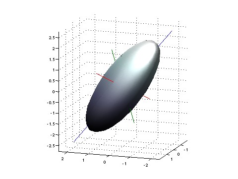
All this is very visual, at least for me. If you imagine the fluctuations as forming a blurry patch near the point 
To understand the covariance matrix, it may help to start by rewriting the variance of a single observable

That’s a lot of angle brackets, but the meaning should be clear. First we look at the difference between our observable and its mean value, namely

Then we square this, to get something that’s big and positive whenever our observable is far from its mean. Then we take the mean value of the that, to get an idea of how far our observable is from the mean on average.
We can use the same trick to define the covariance of a bunch of observables 

If you think about it, you can see that this will measure correlations in the fluctuations of your observables.
An interesting difference between classical and quantum mechanics shows up here. In classical mechanics the covariance matrix is always symmetric — but not in quantum mechanics! You see, in classical mechanics, whenever we have two observables 

since observables commute. But in quantum mechanics this is not true! For example, consider the position 


so taking expectation values we get

So, it’s easy to get a non-symmetric covariance matrix when our observables

You can check that the matrix entries here are the second derivatives of the partition function:

And now for the cool part: this is where information geometry comes in! Suppose that for any choice of values
Then for each point
we have a matrix

And this matrix is not only symmetric, it’s also positive. And when it’s positive definite we can think of it as an inner product on the tangent space of the point 

I hope you can see through the jargon to the simple idea. We’ve got a space. Each point
Now if you look at the Wikipedia article you’ll see a more general but to me somewhat scarier definition of the Fisher information metric. This applies whenever we’ve got a manifold whose points label arbitrary mixed states of a system. But Crooks shows this definition reduces to his — the one I just described — when our manifold is
More precisely: both Crooks and the Wikipedia article describe the classical story, but it parallels the quantum story I’ve been telling… and I think the quantum version is well-known. I believe the quantum version of the Fisher information metric is sometimes called the Bures metric, though I’m a bit confused about what the Bures metric actually is.
[Note: in the original version of this post, I omitted the real part in my definition 


Although a different application (mathematical finance), this reminds me a bit of what I wrote here:
Einstein meets Markowitz: Relativity Theory of Risk-Return
Interpreting covariance as an inner product provides a lot of insight into applied statistics, e.g.
Visualizing Market Risk: A Physicist’s Perspective
But I’ve never seen the added bit that makes it Lorentzian. Any stochastic process has both a stochastic (the part the wiggles around) and deterministic component. I wonder if there is an information theoretic interpretation of the deterministic part?
I haven’t seen a Lorentzian application, but sometimes come across causal correlation (or at least temporal). No, that’s not a joke. It’s exactly the same g_{ij}, but now X_i is a fuction of t_i and X_j(t_j).
Do you have a reference? I think I’ve been needing to reinvent that idea for a problem I’m working on.
Sorry, nothing good in the way of nonequilibrium thermodynamics or anything. I walked out of a nonequilibrium class 25 years ago and haven’t looked back. The occasion was the lecturer pondering deriving that the temperature fluctation was identically zero, after assuming it was nonzero a couple equations earlier. Our text, which we didn’t follow, was Kubo, Toda, and Hashitsume II.
I basically do applied analysis of other people’s data, and one main kind is change detection. In environmental contexts, an example I liked from a few years back was correlating the change in salinity in Gulf of Mexico marshes to later changes in pigment of neighboring areas to predict marshland losses. The presenters were from Tulane and Louisiana State University, but my memory fails besides. For theory of these sorts of causal investigations, delay difference equations are common. I think those are mostly used in network analyses, which I don’t do, but there are plenty of references.
In other applications which I won’t belabor the spatiality/neighborhood aspect is extremely unimportant. We just look for changes in one signal preceding changes in another signal.
Onsager may have arrived firstest with the mostest. Eqs 1 etc in
http://prola.aps.org/pdf/PR/v38/i12/p2265_1
I’ll come out and admit that I never ever have heard of the Bures metric, although it would seem that it was introduced in 1969. Wikipedia does not offer a hint if anyone did anything interesting with it…
A side note:
JB is deliberately simplifying matters. This is true in the case where we assume that the spectrum of the density matrix consists of eigenvalues only. This need not be the case of course. In the more general setting we’d need to use (holomorphic) functional calculus to define the value of a function of a (positive) operator :-)
John wrote:
Tim wrote:
Right. But note: this is always true for a density matrix: a density matrix has finite trace, so its spectrum must consist of eigenvalues only! So I should have said “density matrix” where I said “positive operator”.
Later I screwed up a bit more: when I defined the exponential of an operator, I was using a definition that’s fine for self-adjoint operators whose spectrum consists of eigenvalues only, but we may want to apply these ideas more generally, and then we need the full-fledged functional calculus. I will correct my statement.
For people reading this and feeling nervous: none of these issues matter if we’re dealing with a quantum system with a finite-dimensional Hilbert space. Then everything I’d said is fine.
Copy-editing note: $\lambda_1, \dots \lambda_n$ and $n \times n$ need the extra “latex” to render properly. Not that we all aren’t used to parsing TeX in our heads, but. . .
Thanks. Fixed!
What we need are really good brain implants that render TeX in an ocular preprocessing unit, so I don’t need to type the bloody “latex” after each dollar sign to get it to work on this blog. (There could in theory be an easier solution, but apparently WordPress hasn’t found it.)
This may be a gedanken idea, or virtual meme, or instance of Dave Berg’s pseudo-Cartesian formulation “I think I’m thinking”, but here’s a leading question anyway. What is the significance of the Berry’s phase of a quantum thermodynamic cycle?
That’s an interesting idea, especially if you compare my description of the Bures metric (which you get when you have a manifold parametrizing mixed states of a quantum system) with my old description of the fidelity metric (which you get when you have a manifold parametrizing pure states).
I hope to have more to say about this — but like you, I’m not sure there’s anything here yet. I have never read about a Berry’s phase for mixed states. There are obvious problems with making it precise.
Wow, ten years ago. “Geometric Phases for Mixed States in Interferometry”
http://prl.aps.org/pdf/PRL/v85/i14/p2845_1
Maybe there has been more recent work.
Okay, here’s something: in
• Anna Jencova, Geodesic distances on density matrices.
the author writes:
The references are these:
[18] A. Uhlmann, Density operators as an arena for differential geometry, Rep. Math. Phys. 33 (1993), 253–263.
[19] A. Uhlmann, Geometric phases and related structures, Rep. Math. Phys. 36 (1995), 461–481.
This should be interesting! Tim van Beek may be interested in the second paper, since it seems to give a general C*-algebraic description of the Bures metric on mixed states.
Is uniqueness true (from Jencova, referenceing Uhlmann): “For each w0 there is a unique w1 parallel to w0”? Uhlmann is over my head.
I just saw this and thought someone here might be interested…
http://news.slashdot.org/story/10/10/22/1236215/Astonishing-Speedup-In-Solving-Linear-SDD-Systems
That’s interesting news indeed! If you like, you could join the azimuth forum and create a thread about numerical mathematics and computer models over there. In addition feel free to add this link e.g. to the climate models page over at the Azimuth project.
In a distant future the numerical and implementation aspects of climate models may be moved to their own pages…but collecting the information that we learn now over there is an important step into that direction :-)
[…] Last time I provided some background to this paper: […]
For the Gibbs state derivation please see http://videolectures.net/mlss05us_dasgupta_ig/
So stupid question maybe, but it is not clear to me why so defined is the real part of the metric.
My problem is the following: by taking the double derivative of , you get a totally symmetrized (and thus Real product of operators):
and it is really not clear to me that that is equal to the real part of the double moment which is
Sorry to take so long to reply to your comment! I got pretty nervous about exactly this point here, but Eric Forgy made feel okay about it in the following comments. So, please look at those, if you haven’t already.
I thought you were going to talk about that Fisher Information Geometry article from Nature a few months ago.
What’s the connection between these Lagrange Multipliers and the ones from calc 3?
And what’s the significance of this being a Riemannian metric, as opposed to any other metric or semi pseudo quasi metric?
Q. P. wrote:
I don’t know about that. If you give me a link, I might say something about it sometime.
They’re exactly the same! We use Lagrange multipliers whenever we want to maximize something subject to some constraints. Here we are trying to maximize entropy
subject to some constraints
Think of as an
as an  self-adjoint matrix that you get to vary, and
  as some fixed self-adjoint matrices. Since the matrix
  has a lot of entries this is a multivariable calculus problem with a lot of variables. To solve it, you need to know a bit about the logarithm of a matrix (which I explained). So, most people taking Calculus 3 couldn’t do this problem, but it’s a great test of ones skill, and it’s fundamental to statistical mechanics.
Well, Riemannian geometry is the math that Einstein used to study curved spacetimes, so a vast amount is known about it. Since I used to work on quantum gravity, I like this branch of math, and I’m eager to see how it applies to the study of information.
For example, there’s a nice theory of geodesics, which are the ‘best approximations to a straight line in a curved space’. In information geometry, it turns out that if you have some data and you want to choose the hypothesis that best fits this data, you sometimes want to draw a geodesic from the probability distribution given by your data to the surface that includes all the hypotheses you’re considering.
That was a pretty vague remark, but later in this series I’ll explain it! So far I’ve written 5 posts in this series, but I’m really just getting started. I quit for a while because I didn’t want it to overwhelm the main point of this blog: how scientists can help save the planet.
[…] Part 1 • Part 2 • Part 3 • Part 4 • Part […]
Gavin Crooks’ paper on “thermodynamic length” helps us understand why relative entropy doesn’t obey the triangle inequality.
Towards the end of the article there is this description of
the Fischer metric as a metric on ‘x_i’ space where these
x_i are averages of the random variables. I always thought
it was the parameter space (lambda_i in the article) which received the metric on its tangent space. Now one may ‘reparametrize’ this space in terms of averages of X_i (which
I am not sure if one can always do). But what makes us want to see it this way?
(Sorry about that part about being unsure. Take the Jacobian
which turns out to be made up of second derivatives of ln(Z)
which is invertible)
[…] is an excellent blog series on information geometry by the renowned mathematician John Baez. I learned a lot from that, but in […]