Summer vacation is over. Time to get back to work!
This month, before he goes to Oxford to begin a master’s program in Mathematics and the Foundations of Computer Science, Brendan Fong is visiting the Centre for Quantum Technologies and working with me on stochastic Petri nets. He’s proved two interesting results, which he wants to explain.
To understand what he’s done, you need to know how to get the rate equation and the master equation from a stochastic Petri net. We’ve almost seen how. But it’s been a long time since the last article in this series, so today I’ll start with some review. And at the end, just for fun, I’ll say a bit more about how Feynman diagrams show up in this theory.
Since I’m an experienced teacher, I’ll assume you’ve forgotten everything I ever said.
(This has some advantages. I can change some of my earlier terminology—improve it a bit here and there—and you won’t even notice.)
Stochastic Petri nets
Definition. A Petri net consists of a set 

saying how many things of each species appear in the input for each transition, and a function
saying how many things of each species appear in the output.
We can draw pictures of Petri nets. For example, here’s a Petri net with two species and three transitions:

It should be clear that the transition ‘predation’ has one wolf and one rabbit as input, and two wolves as output.
A ‘stochastic’ Petri net goes further: it also says the rate at which each transition occurs.
Definition. A stochastic Petri net is a Petri net together with a function

giving a rate constant for each transition.
Master equation versus rate equation
Starting from any stochastic Petri net, we can get two things. First:
• The master equation. This says how the probability that we have a given number of things of each species changes with time.
• The rate equation. This says how the expected number of things of each species changes with time.
The master equation is stochastic: it describes how probabilities change with time. The rate equation is deterministic.
The master equation is more fundamental. It’s like the equations of quantum electrodynamics, which describe the amplitudes for creating and annihilating individual photons. The rate equation is less fundamental. It’s like the classical Maxwell equations, which describe changes in the electromagnetic field in a deterministic way. The classical Maxwell equations are an approximation to quantum electrodynamics. This approximation gets good in the limit where there are lots of photons all piling on top of each other to form nice waves.
Similarly, the rate equation can be derived from the master equation in the limit where the number of things of each species become large, and the fluctuations in these numbers become negligible.
But I won’t do this derivation today! Nor will I probe more deeply into the analogy with quantum field theory, even though that’s my ultimate goal. Today I’m content to remind you what the master equation and rate equation are.
The rate equation is simpler, so let’s do that first.
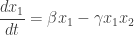
The rate equation
Suppose we have a stochastic Petri net with 


It’s really a bunch of equations, one for each 
The right-hand side is a sum of terms, one for each transition in our Petri net. So, let’s start by assuming our Petri net has just one transition.
Suppose the 


where 
That’s really all there is to it! But we can make it look nicer. Let’s make up a vector

that says how many things there are of each species. Similarly let’s make up an input vector
and an output vector

for our transition. To be cute, let’s also define

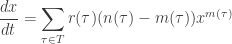
Then we can write the rate equation for a single transition like this:

Next let’s do a general stochastic Petri net, with lots of transitions. Let’s write 


For example, consider our rabbits and wolves:
Suppose
• the rate constant for ‘birth’ is 
• the rate constant for ‘predation’ is 
• the rate constant for ‘death’ is 
Let 


If you stare at this, and think about it, it should make perfect sense. If it doesn’t, go back and read Part 2.
The master equation
Now let’s do something new. In Part 6 I explained how to write down the master equation for a stochastic Petri net with just one species. Now let’s generalize that. Luckily, the ideas are exactly the same.
So, suppose we have a stochastic Petri net with 


To keep the notation clean, let’s introduce a vector
and let

Then, let’s take all these probabilities and cook up a formal power series that has them as coefficients: as we’ve seen, this is a powerful trick. To do this, we’ll bring in some variables 

as a convenient abbreviation. Then any formal power series in these variables looks like this:
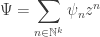
We call 

The simplest example of a state is a monomial:

This is a state where we are 100% sure that there are
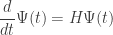
The master equation says how a state evolves in time. It looks like this:

So, I just need to tell you what 
It’s called the Hamiltonian. It’s a linear operator built from special operators that annihilate and create things of various species. Namely, for each state

and a creation operator:

How do we build

where as usual we’ve introduce some shorthand notations to keep from going insane. For example:

and
Now, it’s not surprising that each transition

How can we understand it? The basic idea is this. We’ve got two terms here. The first term:

describes how 


is a bit harder to understand, but it says how the probability that nothing happens—that we remain in the same pure state—decreases as time passes. Again this happens due to our transition
In fact, the second term must take precisely the form it does to ensure ‘conservation of total probability’. In other words: if the probabilities 
Let’s look at an example. Consider our rabbits and wolves yet again:
and again suppose the rate constants for birth, predation and death are

where

and 
where the Hamiltonian is

and 


In each case, the first term is easy to understand:
• Birth annihilates one rabbit and creates two rabbits.
• Predation annihilates one rabbit and one wolf and creates two wolves.
• Death annihilates one wolf.
The second term is trickier, but I told you how it works.
Feynman diagrams
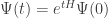
How do we solve the master equation? If we don’t worry about mathematical rigor too much, it’s easy. The solution of
should be
and we can hope that

so that

Of course there’s always the question of whether this power series converges. In many contexts it doesn’t, but that’s not necessarily a disaster: the series can still be asymptotic to the right answer, or even better, Borel summable to the right answer.
But let’s not worry about these subtleties yet! Let’s just imagine our rabbits and wolves, with Hamiltonian
Now, imagine working out

We’ll get lots of terms involving products of 

And suppose we want to compute

as part of the task of computing 

We can draw this as a sum of Feynman diagrams, including this:

In this diagram, we start with one rabbit and one wolf at top. As we read the diagram from top to bottom, first a rabbit is born (
This is just one of four Feynman diagrams we should draw in our sum for 

will involve a lot of Feynman diagrams… and of course computing

will involve even more, even if we get tired and give up after the first few terms. So, this Feynman diagram business may seem quite tedious… and it may not be obvious how it helps.
But it does, sometimes!
Now is not the time for me to describe ‘practical’ benefits of Feynman diagrams. Instead, I’ll just point out one conceptual benefit. We started with what seemed like a purely computational chore, namely computing

But then we saw—at least roughly—how this series has a clear meaning! It can be written as a sum over diagrams, each of which represents a possible history of rabbits and wolves. So, it’s what physicists call a ‘sum over histories’.
Feynman invented the idea of a sum over histories in the context of quantum field theory. At the time this idea seemed quite mind-blowing, for various reasons. First, it involved elementary particles instead of everyday things like rabbits and wolves. Second, it involved complex ‘amplitudes’ instead of real probabilities. Third, it actually involved integrals instead of sums. And fourth, a lot of these integrals diverged, giving infinite answers that needed to be ‘cured’ somehow!
Now we’re seeing a sum over histories in a more down-to-earth context without all these complications. A lot of the underlying math is analogous… but now there’s nothing mind-blowing about it: it’s quite easy to understand. So, we can use this analogy to demystify quantum field theory a bit. On the other hand, thanks to this analogy, all sorts of clever ideas invented by quantum field theorists will turn out to have applications to biology and chemistry! So it’s a double win.


Typo: The first “creation operator” is the annihilation operator.
Thanks! I can never make up my mind which deserves to come first: annihilation or creation. Here I changed my mind but forgot to fix everything.
There’s a certain naive sense in which creation must come before annihilation. And logically speaking, creation is more fundamental than annihilation, since in the Bargmann-Segal approach the creation operator comes from quantizing the function on the classical phase space
  , while the annihilation operator comes from quantizing the function
  . We can also see this, sort of, in the fact that the creation operator, multiplication by
  , is simpler than the annihilation operator,
  . So, my advisor Irving Segal called the creation operator
  and called the annihilation operator
  .
.
That’s logical, but nobody followed him… not even me. Like everyone else, I write the annihilation and creation operators as
  and
and  . So, I should always say “annihilation and creation”, not “creation and annihilation”. But sometimes I slip.
This reminds me of Cartier’s interesting Mathemagics paper:
http://www.emis.de/journals/SLC/wpapers/s44cartier1.html
By the way, aren’t there constants missing when you simplify the composite of creation and annihilation operators in the rabbit example? Similarly, you say that the second term in the master equation does “nothing”.
Hi, Dan! We could use a bit more mathemagic in biology, chemistry and other subjects… and maybe we can simultaneously see that Feynman diagrams aren’t quite so magical.
I don’t quite understand—what constants are missing where? When I said:
I was deliberately leaving out a bunch of constants, since this term appears when we compute
But I don’t recall “simplifying the composite of creation and annihilation operators in the rabbit example”. I could have made a typo.
Dan wrote:
No, I said “it says how the probability that nothing happens—that we remain in the same pure state—decreases as time passes.” So, it doesn’t do nothing, it describes the rate at which nothing having happened decreases!
Jacob explained this back in Part 7. For example, consider a single species: amoebas. If there’s a certain probability per unit time for an amoeba to reproduce, you might think the Hamiltonian was
but this is just the first term, which describes the rate per unit time at which one amoeba turns into two. This process increases the probability that there’s one more amoeba… but that means the probability that there’s the same number of amoebas must decrease! That decrease is described by the second term
If we apply the whole Hamiltonian
to a state with
with  amoebas, we get
The number shows up because
we call the number operator for this reason.
But more importantly, all this stuff makes sense. The rate at which the probability of having one more amoeba grows is … so this must be the rate at which the probability of having the same number of amoebas decreases.
I know you know most of this stuff… I’m just using your question as an excuse to clarify this mildly confusing issue. Anyway, we see that doesn’t do ‘nothing’ to
  ; it describes the rate at which the probability that nothing has happened decreases!
This issue was the main thing that confused me when I reinvented this whole theory. I think some of the confusion arises from the fact that we don’t tend to think much about ‘the rate at which the probability that nothing has happened decreases’.
Sorry for not being more specific. The thing I’m confused about is that the formula you give for is
is
But shouldn’t the -1 really be i.e. the number operator? That’s the “constant” I was referring to.
Yes, you’re right, Dan. That was just a dumb mistake on my part—or, maybe I can pretend it was a typo.
Fixed!
By the way, as you may have noticed, your LaTeX didn’t work because you forgot that on WordPress blogs, you need to write your equations like this:
$latex E = mc^2 $
with the word ‘latex’ directly after the first dollar sign, no space between them. Also, double dollar signs don’t work.
But if you think that’s bad, just think what I had to do to make you see
$latex E = mc^2 $
If I’d typed what you see, you’d have seen
The only way out was for me to look up the HTML for a dollar sign!
Dan wrote:
It’s a splendid article. In a way the duality exposed is the ‘platonist while working’, ‘formalist when asked’ duality. It is also the difference between the way mathematics is done and the way it is presented in papers. So I think this is really a plea for greater honesty by mathemeticians about ‘works in progress’ – sharing their ideas earlier, so that others can assist in the development, before everything gets wrapped up, neat and tidy.
Quick note: your first “creation operator” in bold should be “annihilation operator”.
Fixed!
I’m interested – will Feynman diagrams truly be a new technique in Petri nets? Was it not used before in this field, perhaps in some different avatar?
I’m in the states and am blogging the night shift. John is not making me work nights this time (see Network Theory 7) — its nearly sun rise where he is in Singapore and he gets to wake up and see this lame post! Good morning John.
I’ll soon be back from my long quantum network hiatus and world tour, to use mathematics to possibly help save the planet and to work 20 hours a day in Singapore to try to keep up with you.
In my own point of view, and as far as I know, there are a few things connecting here. (i) Chemical reaction networks, (ii) Petri networks, (iii) Feynman diagrams and some other stuff too.
Again, from my own point of view, its more important at this stage to figure out how to unite everything into a unified theory. This would allow people to cast any of the techniques they wished from one field into the other. We will figure out what these established methods are going to tell us. One of the great method from quantum mechanics is Feynman diagrams — these have appeared in the blog articles, as a very intuitive way to explain this stuff.
Its hard to sell new tools to people if you can’t say what they are good for. So one of the things several people are trying to do right now is to find some research papers where some of the theorems from one field now apply to another, based on John’s mappings, but this is another story (get ready for Brendan Fong). Its just conjecture at this stage in the game to say, “Feynman diagrams are going to rock the Petri net world!”
Bruce wrote:
I’ve never seen people use the phrases ‘stochastic Petri net’ and ‘Feynman diagram’ in the same sentence before. That connection could be my discovery. But if so, it’s nothing to be proud of. It’s mainly because the Petri net community is cut off from other communities who are studying the exact same ideas!
The idea of using quantum field theory techniques in ‘stochastic field theories’ is not new… and these theories are really just stochastic Petri nets of an elaborate sort.
After my first discussion of this subject, Blake Stacey dumped a ton of references on us. He wrote:
I didn’t know any of this stuff when I came up with the ideas I’ve been presenting so far. But again, that’s nothing to be proud of. So far in this series I haven’t done anything profoundly new: I’m mainly just trying to explain the relation between quantum mechanics and stochastic mechanics.
However, I think understanding that relation better will let us do some new things.
That last paper above by Dodd and Ferguson seems to proceed quite far along the path you are advocating (Feynman diagrams to study stochastic Petri nets). They get to “effective actions”, “one loop approximations”, etc.
But fair enough, it is a recent paper (2009), and it seems like they wrote it as the start of a new exciting research direction. I guess they should be invited to the Banff workshop you are proposing.
In case anyone’s wondering, when I said this:
I was mainly referring to how I’m now calling those yellow circles in Petri nets species rather than states. ‘State’ is an irresistible term for something else: the probability distribution , which evolves according to a stochastic version of Hamilton’s equations! And, in both population biology and chemistry, the different species in our Petri net really are called ‘species’.
For species in chemistry, see this.
By the way, if anyone wants to see the whole “Network Theory” series with prettier equations, go here:
• Network theory.
It seems people use Petri net techniques in ecology. You’d imagine there that you want to include extra information, e.g., at Birth one rabbit continues and a baby is born; Death for wolves is age dependent, as is Predation; rabbits who survive an attack are wiser, and so on. Identity through transitions matters.
Hi, David! Thanks for the link!
I believe if you want to think of animals as distinguishable particles, you should either not use the formalism I’m talking about here (which treats particles as indistinguishable, albeit classical rather than quantum), or introduce more species in the Petri net.
For example, instead of just ‘rabbit’, we can have ‘dumb young bunny’ and ‘wise old hare’. Then we can have two transitions in which a dumb young bunny is attacked by a wolf: one in which the dumb young bunny is merely annihilated, another in which it’s transformed into a wise old hare. If that’s too simple, we can have various degrees of wisdom, and more kinds of attacks.
This may seem clunky, but it’s really exactly like equipping elementary particles with ‘spin’ and other ‘internal degrees of freedom’, which can change in interactions. With the right notation it’s not messy.
Similarly, instead of having just ‘wolf’, we can have ‘1-year old wolf’, ‘2-year old wolf’ and so on. Unfortunately, the stochastic Petri net would have wolves randomly getting older, instead of deterministically getting older!
One way around this is to generalize the master equation so that it involves ‘explicit time-dependence’, rather than a time-independent Hamiltonian.
Again, this kind of thing is familiar from quantum physics. Without a explicitly time-dependent Hamiltonian, it’s hard to make particles have an ‘inherent age’. To a very good approximation, for example, an ‘old’ radioactive atom is no more likely to decay (per unit time) than a ‘young’ freshly formed one.
(There are some astounding subtleties here, contained in the phrase ‘to a very good approximation’.)
Anyway, as one cranks up the level of detail one wants from ones model, eventually one will decide that stochastic Petri nets are not sufficiently flexible… but I’m going to continue playing with them for now!
There’s another set of experiments with modelling a predation example on this Azimuth page. It might be mildly interesting in how it handles separate population aging. (Partly because I’m primarily interested in applying experimental mathematics, particularly since since if there are as many tipping points nearby as people think, the “extraction” of ideas from data rather than “bottom-up logic” may become equally important. So I’m deliberately choosing a slightly different approach to the one John, Jacob and Brendan are working in not because I have any problems with their approach, but viewing this as having the same relationship “experimental mathematics number theory” has to “number theory”, i.e., different types of attack on the area.
Unfortunately I’ve spent most of the time over the past couple of months accommodation hunting limiting my free time, and in one week’s time I’ll be going effectively internetless for an unknown numbers of weeks until I move into my new accommodation, so little progress has been made on the codebase up on the Azimuth code project, although I’ve been developing ideas.
I should add that people also study ‘colored’ Petri nets, where the little ‘tokens’ representing things of a given species aren’t all black like this:
but instead come in different ‘colors’. This gives the tokens a certain limited amount of ‘individual identity’, though two tokens of the same color and the same species are indistinguishable.
People who remember the category-theoretic interpretation of Petri nets may enjoy thinking about what we’re doing here.
Back here you wrote
I wonder what effect colouring the ignored tokens has on the category-theoretic interpretation.
By the way, did you ever see Abramsky’s Petri Nets, Discrete Physics, and Distributed Quantum Computation?
As we saw in Part 8, any stochastic Petri net gives two equations: the rate equation and the master equation […]
[…] Here’s the general form of the rate equation: […]
Hi,
I’m trying to fully understand the Feynman diagram drawn above for the rabbit/wolf interaction and I have a few questions:
Let’s consider the first order approximation, i.e.
Using the creation and annihilation operators for this system, we write down that to this order,
where means there are m rabbits and n wolves and we started in a state with one of each. We learned in post 5 that the mapping by a stochastic operator must preserve the sum of
probabilities, i.e using your notation
So does this mean a time dependent normalization constant must be introduced in the above equation for the ? i.e if we wanted to know what the probability is of finding 2 rabbits and 1 wolf at some time
  , in this first order approximation, is it correct to say that
?
Thanks,
Nick
Hi! I’m glad you’re trying to understand this stuff, and asking questions.
We should not need an extra time-dependent normalization factor: the formula
should really be correct to first order in without any fudge factors.
I think the problem is this: you’re not using the whole Hamiltonian in your calculation. As I explained in the post, the Hamiltonian is
where
The terms with minus signs in front are crucial: these serve to ensure that is stochastic, meaning:
If you leave these terms out, you won’t be reducing the probability that the system stays in its old state as you increase the probability that it’s in some new state. Then the sum of the probabilities won’t stay equal to one… and that’s why you were tempted to try other tricks, like time-dependent normalization constants, to force it to stay equal to one!
When I was first (re)discovering this stuff, these terms with minus signs were the most mysterious and fascinating aspect of the whole subject. I explained them in Part 6, so you might want a look at that.
Lightbulb!
Thanks, got it now.
I’m trying to understand the sense in which the stochastic Petri nets are the same concept or a variant concept from other treatments that I read about stochastic Petri nets. So essentially my question that follows is terminological, not substantive. My motivation is that I am writing a blog article, and so I want to get clear about what the terms mean.
The treatments that I see for “stochastic Petri nets” define them as basic Petri nets, along with a probability distribution function for the intervals between firing events — which is taken, in the vanilla model, to be an exponential distribution, because this is what satisfies the “memoryless” property for the waiting time between transitions.
So to combine this with the mass action kinetics, you would multiply the rate constant for the transition with the products of the concentrations of the input species, to determine the expected firing rate of the transition in a given state, and use this as the rate parameter for the exponential distribution, to obtain the distribution of expected intervals for that transition at that time in the given state of the net.
In your definition of stochastic Petri nets, you specify only a rate constant for each transition, with no mention being made of the distribution of firing intervals.
I believe that this is related to the that was raised on the forum by Tim van Beek, which you quoted him as saying: Where is the probability space?
Your answer was: “I don’t need to hide the truth: our measure space is ℕ^k, where k is the number of states in our Petri net. A point in ℕ^k tells us how many things there are in each state. A stochastic Petri net determines a Markov chain on this measure space.”
That is fine, but I just wanted to confirm that you are working with an essentially different kind of “stochastic Petri net” than the ordinary treatments of the matter. The probability distributions that are are working with, and which are operative in the master equation, look like states of belief concerning the marking of the net. You haven’t defined any probability distribution pertaining to the underlying random process that is physically driving the reactions in the network.
Not that you should have done so. I’m just trying to clarify the nomenclature, so that I don’t introduce confusion when I myself write about the subject.
If what I say here is correct, I am reluctant to define a Petri net that has only rate constants as a stochastic Petri net — notwithstanding the fact that one can do very fine stochastic work with the master equations, Hamiltonians, etc. — because of the terminology clash with existing literature. Is there a name for “Petri nets plus rate constants plus the mass action kinetics,” which is indeed sufficient to introduce the rate equations, and to serve as the basis for the “stochastic mechanics” that you successfully develop.
David wrote:
No, they’re exactly the usual ones. Maybe I’m explaining them in a way that looks different, but I just read about the usual ones and then started explaining them.
Try this, for example:
• M. A. Marsan, Stochastic Petri nets: an elementary introduction.
The definition on page 12 is almost the same as mine except for the names of things. There are a couple of differences. It includes an ‘initial marking’ assigning a natural number to each species. This just gives the stochastic Petri net a definite state to start out in. Also, he allows the firing rates to be marking dependent, while I don’t… but he does so parenthetically, and it seems that in general he doesn’t exploit this option.
The book where I first learned about stochastic Petri nets gave, I believe, a definition that exactly matches the one I’m using, except for the names of things:
• Darren James Wilkinson, Stochastic Modelling for Systems Biology, Taylor and Francis, New York, 2006.
There’s lots of slight variations in the Petri net terminology; it hasn’t settled down as much as terminology in say, group theory. Given this, I think I’m being surprisingly orthodox in my use of terminology. My main innovation is to exploit the isomorphism between (my) stochastic Petri nets and the chemist’s ‘chemical reaction networks’ and try to use the same terms whenever possible in both subjects.
Ok, thanks for the references and the clarification. The Wilkinson book sounds interesting and I have ordered it.
John wrote:
From my reading it looks like both you and Marsan use marking dependent firing rates. For you it is the product of the rate constant times the species concentrations. For him the firing rates are part of the given data.
By the way I found some useful information here in this survey article:
• David F. Anderson and Thomas G. Kurtz, Continuous time Markov chain models for chemical reaction networks
David wrote:
Oh, okay. If ‘firing rate’ means the probabilistic rate at which a given transition occurs, you’re right: for me, this is the product of the rate constant and the products of the concentrations of the various species that appear as inputs to the transitions. (The usual law of mass action.)
But with this definition of firing rate, it’s impossible for the firing rates to be independent of the markings: otherwise we’d be in the untenable position of saying that transitions can occur at nonzero rates even because the necessary input species aren’t present!
(Well, okay, it’s possible—but only if the firing rates are all zero.)
This is one reason I had interpreted ‘firing rates’ to mean ‘rate constants’, which is probably wrong.
Thanks for the extra reference. Anderson and Kurtz are two architects of the wonderful Anderson–Craciun–Kurtz theorem.
By the way, when are you gonna get that blog post done? I bet you’re overthinking it. Anything that takes a really long time to write is probably too deep for anyone to understand in the amount of time most people are willing to spend reading a blog post.
Hi, involves the computation of a lot of Feynman diagrams (all possible). I was trying to understand the physical meaning of
In the section on Feynman diagrams, you say that finding
in terms of these.
First of all if we simply operate with on
on  , then we get
  which then gives
  . The second and fourth factors were a little confusing. They come because the probability of
  decreases after B. Is it because, were there any remaining
  after B, they would have led to
  after operation with C?
In
I was thinking of this as the sum of probabilities of all possible courses of events to get to the expected . What is the physical significance of having a factor of
  in the nth term ? Shouldn’t the probability of having 3 events in succession simply be proportional to
  – why the extra factor of
  ?
?
Arjun wrote:
I always find these negative terms a bit hard to explain, but the key is that the sum of probabilities must equal 1, so if some probabilities increase, others must decrease. In stochastic mechanics the vector is a way of describing a list of probabilities, and the master equation
says how these probabilities change. Since some of these probabilities must decrease if others increase, we know that some of the coefficients in must be negative. You can understand the negative coefficients this way.
The way I like to summarize it is this: the probability of staying in the same state goes down at the same rate the probability of being in another state goes up.
It may be helpful to think about the simplest example, where there’s just one species and the Hamiltonian is
for some rate constant
Suppose it’s raining and you count the raindrops hitting a table outdoors. Suppose you find that on average the number of raindrops per second hitting the table is Then the probability that
  raindrops hit the table in
  seconds is
We figured this out in Part 5. You can also work it out by computing
This should help you see where the factors of come from, and why they’re necessary and natural.
I’ve been trying to get from the master equation to the rate equation. As a starting example, I considered a simple net consisting of one species and one transition with n=4 and m=2, and rate constant r.
Now the master equation says that where
where  .
.
Operating with on both sides, then writing everything in terms of n and then putting z=1, we get
 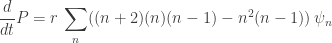 , where P is the expected value of n.
As is required in the rate equation, n is large. Therefore, .
.
Now, the actual rate equation is , i.e.
  .
.
Therefore, we’ll get the required result if the variance if zero. In similar examples with higher n,m we require higher moments to be 0 also. What is the significance of this?
Also, for the general case of multiple species, what is the form of N in terms of annihilation and creation operators, to get the expected value?
Arjun wrote:
Great! In our seminar at UCR last quarter we spent a few sessions doing this. I am now writing a paper about what we discovered, called “Quantum techniques for studying the large number limit in chemical reaction networks”. I hope to be done in a couple weeks. If I didn’t already know many of the main results, I’d suggest this as a topic for you to work on when we meet in Singapore. Even though I do know many of the main results, there might be other things left to do.
Or more generally: if the variance is smaller than some number, we get the rate equation to within some accuracy. This sort of “for every there is a
  ” formulation is more useful, since it’s unlikely for the variance to be exactly zero.
Right! Of course if the variance is zero so are these higher moments. But more generally, we need estimates on these higher moments to obtain the rate equation to within some given accuracy.
I don’t know, it just makes a lot of sense that you need bounds on higher moments of if you are dealing with process with more inputs, since those involve terms like
There’s one number operator for each species,
It counts how many things we have of the $i$th species.
Luca Cardelli is interested in chemical reaction networks actually found in biology. This approximate majority algorithm is seen quite clearly in a certain biological system: a certain ‘epigenetic switch’. However, it is usually ‘obfuscated’ or ‘encrypted’: hidden in a bigger, more complicated chemical reaction network. For example, see:
• Luca Cardelli and Attila Csikász-Nagy, The cell cycle switch is approximate majority obfuscated, Scientific Reports 2 (2012).
This got him interested in developing a theory of morphisms between reaction networks, which could answer questions like: When can one chemical reaction network (CRN) emulate another? But these questions turn out to be much easier if we use the rate equation than with the master equation. So, he asks: when can one CRN give the same rate equation as another?
I’m confused about the interpretation of the master equation in the case that one species is much rarer than another. Katie Casey and I have been discussing this quite a bit without finding a resolution; maybe someone here can help us out.
Suppose there are species ,
,  and
and  , and two reactions with the same rate constants:
  , and
, and  . Now, let’s think intuitively about this. Surely the requirements for reaction B to occur are strictly more stringent than those for reaction A: while A requires only an
  , B requires an
  and a
and a  . If we imagine our
  ,
,  and
and  molecules rushing around in a liquid, reaction A can occur any time, on any
  present; but reaction B is restricted to occurring when molecules
  and
and  are in close contact.
To make this distinction most extreme, consider the case that there are many molecules — say, 1000 of them — and just one
  molecule. Then at any particular moment, there are 1000 chances for reaction A to take place, but at most 1 chance for reaction B to take place, since there’s only 1
  molecule present. So intuitively, since reactions A and B have the same rate constants, we might expect the observed rates of A and B to be in a ration of 1000 to 1.
Now, let’s analyze this situation with the master equation, which predicts that when the number of each species is well-defined, the rate at which a particular reaction takes place is given by the rate constant, multiplied by, for each input species, the number of that species present. (This is only exactly correct when each the reaction input involves at most 1 of each species.)
So, let’s analyze the situation with 1000 molecules and 1
  molecule. Since
  , we see that reactions A and B will take place at an equal rate, violating the intuitive ratio derived above by a factor of 1000.
Worse, I argued above that whatever the physical state, reaction B should take place less often than reaction A, since it has more stringent preconditions. But this is also not predicted by the master equation. In a state with 1000 molecules and 1000
  molecules, the master equation predicts that reaction B will take place at a rate of
  , which is 1000 times more often than reaction A.
Why does this make sense? What microphysical interpretation of the underlying physics makes this reasonable? What is so flawed about the intuitive argument described above?
I have trouble understanding what you’re worrying about. It seems you’re saying that getting bitten by a mosquito has more stringent preconditions than spontaneously combusting, since you can spontaneously catch on fire all by yourself, but to get bitten you also need a mosquito. But no mattter how unlikely it is that one mosquito will bite you in a second, and no matter how likely it is to spontaneously combust, if you’re in a room with enough mosquitoes you’ll probably get bitten first.
(This assumes a ‘well mixed’ situation, where all the mosquitoes get an equal chance to bite you. If there are of them, the expected time for the first one to bite goes roughly as
  )
)
Hi John, thanks for your reply. In the situation you describe, I would say that the rate constants for the two processes should be very different to each other. But in my example, it was important that the rate constants were the same.
It’s not quite clear to me how the rate constant ought to be defined physically, but maybe it’s something like this: the reciprocal of the expected time until the process occurs, when the initial state is given exactly by the input molecules required by the process, and no other process can take place.
So, what should the rate constant for spontaneous combustion be, by this definition? Let’s say 1/(1000 years). But for getting bitten by a mosqito, 1 per minute would probably be about right.
I was going to change “spontaneous combustion” to “sneezing”, to get around this objection, but I didn’t do it in time.
That sounds right. It’s good to think about numerically simulating a stochastic Petri net or (equivalently) chemical reaction network using the ‘Gillespie algorithm’. Since Wikipedia explains that algorithm in the case of a reversible reaction
A + B → AB
AB → A + B
I think I won’t explain it.
Actually, there’s an even simpler and conceptually clearer, but less efficient, algorithm in which you increment the time by a very small amount Δ in each step. Then the chance that a given reaction occurs in that step will be Δ times the rate constant times the number of ways that reaction can occur (some obvious product involving the number of molecules of each type involved in that reaction).
If Δ is small enough, the chance that two different reactions occur in a given time step becomes negligible, so we can ignore that possibility, and the annoying issue of ‘deadlocks’, where doing one reaction makes it impossible to do another reaction, and vice versa, since there’s not enough stuff around to do both.
So, we just keep incrementing the time and randomly either doing one reaction or no reaction. The inefficiency is that you spend most of your time doing nothing. The Gillespie algorithm gets around that problem.
OK, let’s use ‘sneezing’ and ‘getting bitten by a mosquito’ as the examples. Suppose they both have a rate constant of 1 per minute, meaning that if one person is left alone in a room by themselves, they will sneeze on average once per minute; and that if a person is left alone in a room with a mosquito, they will get bitten on average once per minute.
Let’s think: why will the mosquito only bite the person once per minute? It must be that the mosquito is buzzing around the room and only encounters the person once per minute, at which point a bite is instantly made, and the mosquito then flies off trying to find another person to bite.
If we have 100 people and 1 mosquito in the room, then the master equation predicts 100 sneezes per minute, and 100 bites per minute. That agrees with the intuition just outlined above.
The problem I had with this is that I thought the master equation assumed that the constituents were ‘well-mixed’ — as if being stirred infinitely fast with an big spoon — ensuring that any subset of molecules would in fact come into contact arbitrarily soon, at least for a small length of time. Coupled with the intuition above, this would mean that even with 1 person and 1 mosquito in the room, there would be an infinite number of bites per minute, unless the bites themselves took some finite amount of time, which was the alternative basis for the rate constants that I was considering.
But I have now spent some time reading Gillespie’s “A rigorous derivation of the chemical master equation”, and I see that this isn’t quite right: rather, we should assume that the molecules move around as if they are particles of an ideal gas at some temperature . The well-mixed assumption just means that the system is kept homogeneous over time. And if we change the temperature of the system, the rate constants would change as well.
Jamie wrote:
That’s one possibility. Another possibility is that it encounters the person more often, but only bites some fraction of the time. In chemical reactions I believe the analogous thing can happen: the reaction isn’t guarantee to happen every time the molecules get close enough.
Are you having stocks and flow in mind?
Are there works which show how the first algorithm (i.e. something like stocks and flow modulo adjustments via taking logarithms and normalizations) and/or (?) the Gillespie algorithm converge in the continuous time limit to the Master equation, at least for examples? By my experience with nonlinear systems especially for longer time spans the quality of convergence may depend quite extremely on the concrete realizations of the flow dependencies.
Nad wrote:
Sort of, but not exactly. The Gillespie algorithm, and the simpler one I described, are random algorithms: they are not deterministic. They are not trying to numerically solve the master equation that describes the change of probabilities with time, they are trying to simulate a specific randomly chosen history of a stochastic process.
A while back you asked what someone meant by ‘a realization’ of a Markov process. What I’m calling ‘a specific randomly chosen history’ is the same thing as a ‘realization’. In the Feynman path integral approach to quantum mechanics it would be called a ‘path’ or a ‘history’, but here we are using the same idea for a stochastic process, not a quantum system. We’re trying to randomly pick one of the possible histories of the world, with the correct probability. It’s an example of a Monte Carlo method.
Someone should prove some theorems about how well these algorithms work, and maybe someone has, but I don’t know those theorems.