The Beauty of Roots

I feel like talking about some pure math, just for fun on a Sunday afternooon.

Back in 2006, Dan Christensen did something rather simple and got a surprisingly complex and interesting result. He took a whole bunch of polynomials with integer coefficients and drew their roots as points on the complex plane. The patterns were astounding!

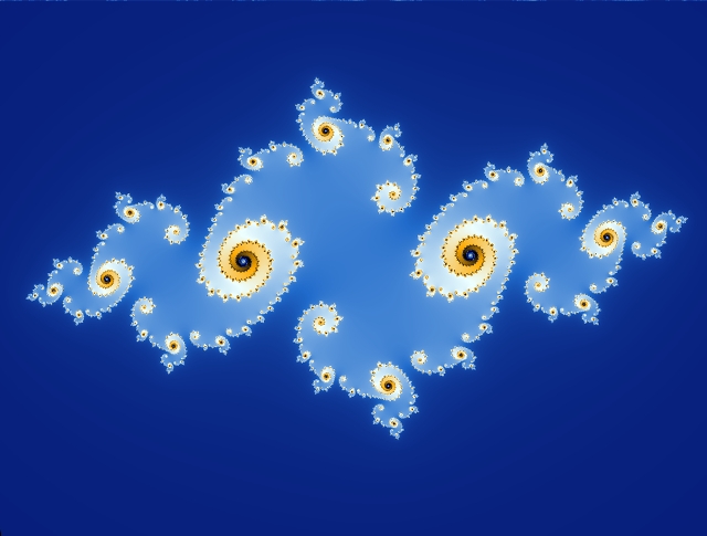
Then Sam Derbyshire joined in the game. After experimenting a bit, he decided that his favorite were polynomials whose coefficients were all 1 or -1. So, he computed all the roots of all the polynomials of this sort having degree 24. That’s 224 polynomials, and about 24 × 224 roots—or about 400 million roots! It took Mathematica four days to generate the coordinates of all these roots, producing about 5 gigabytes of data.

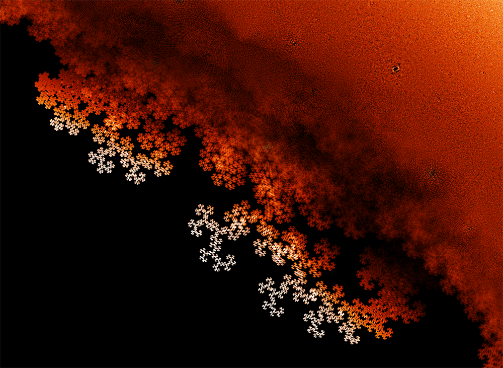
He then plotted all the roots using some Java programs, and created this amazing image:

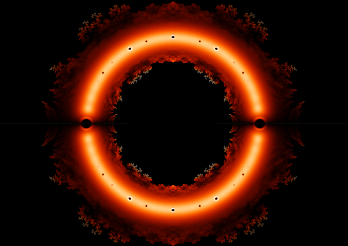
You really need to click on it and see a bigger version, to understand how nice it is. But Sam also zoomed in on specific locations, shown here:


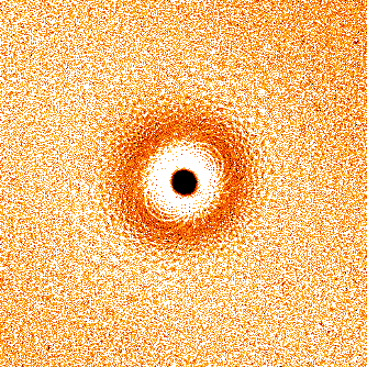
Here’s a closeup of the hole at 1:

Note the line along the real axis! It’s oddly hard to see on my computer screen right now, but it’s there and it’s important. It exists because lots more of these polynomials have real roots than nearly real roots.

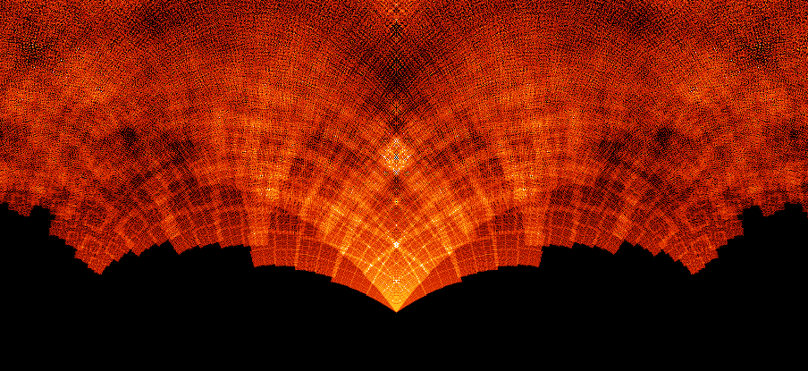
Next, here’s the hole at i:


And here’s the hole at e^{i \pi / 4}:

Note how the density of roots increases as we get closer to
this point, but then suddenly drops off right next to it. Note also the subtle patterns in the density of roots.

But the feathery structures as we move inside the unit circle are even more beautiful! Here is what they look near the real axis — this plot is centered at the point \frac{4}{5}:

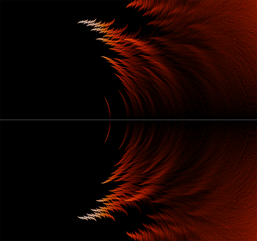
They have a very different character near the point \frac{4}{5}i:

But I think my favorite is the region near the point \frac{1}{2}e^{i/5}. This image is almost a metaphor of how mathematical patterns emerge from confusion… like sharply defined figures looming from the mist as you drive by with your headlights on at night:

Now, you may remember that I said all this already in “week285” of This Week’s Finds. So why am I talking about it again?

Well, the patterns I’ve just showed you are tantalizing, and at first quite mysterious… but ‘some guy on the street’ and Greg Egan figured out how to understand some of them during the discussion of “week285”. The resulting story is quite beautiful! But this discussion was a bit hard to follow, since it involved smart people figuring out things as they went along. So, I doubt many people understood it—at least compared to the number of people who could understand it.

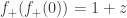
Let me just explain one pattern here. Why does this region near \frac{1}{2}e^{i/5}:

look so much like the fractal called a dragon?

You can create a dragon in various ways. In the animated image above, we’re starting with a single horizontal straight line segment (which is not shown for some idiotic reason) and repeatedly doing the same thing. Namely, at each step we’re replacing every segment by two shorter segments at right angles to each other:

At each step, we have a continuous curve. The dragon that appears in the limit of infinitely many steps is also a continuous curve. But it’s a space-filling curve: it has nonzero area!

Here’s another, more relevant way to create a dragon. Take these two functions from the complex plane to itself:

\displaystyle{ f_+ (x) = \frac{1+i}{2} x }

\displaystyle{ f_- (x) = 1- \frac{1-i}{2} x }

Pick a point in the plane and keep hitting it with either of these functions: you can randomly make up your mind which to use each time. No matter what choices you make, you’ll get a sequence of points that converges… and it converges to a point in the dragon! We can get all points in the dragon this way.

But where did these two functions come from? What’s so special about them?

To get the specific dragon I just showed you, we need these specific functions. They have the effect of taking the horizontal line segment from the point 0 to the point 1, and mapping it to the two segments that form the simple picture shown at the far left here:

As we repeatedly apply them, we get more and more segments, which form the ever more fancy curves in this sequence.

But if all we want is some sort of interesting set of points in the plane, we don’t need to use these specific functions. The most important thing is that our functions be contractions, meaning they reduce distances between points. Suppose we have two contractions f_+ and f_- from the plane to itself. Then there is a unique closed and bounded set S in the plane with

S = f_+(S) \cup f_-(S)

Moreover, suppose we start with some point x in the plane and keep hitting it with f_+ and/or f_-, in any way we like. Then we’ll get a sequence that converges to a point in S. And even better, every point in S show up as a limit of a sequence like this. We can even get them all starting from the same x.

All this follows from a famous theorem due to John Hutchinson.

“Cute,” you’re thinking. “But what does this have to do with roots of polynomials whose coefficients are all 1 or -1?”

Well, we can get polynomials of this type by starting with the number 0 and repeatedly applying these two functions, which depend on a parameter z:

f_+(x) = 1 + z x

f_-(x) = 1 - z x

For example:

f_+(0) = 1

f_+(f_+(0)) = 1 + z

f_-(f_+(f_+(0))) = 1 - z(1 + z) = 1 - z - z^2

f_+(f_-(f_+(f_+(0)))) = 1 + z(1 - z - z^2) = 1 - z - z^2 + z^3

and so on. All these polynomials have constant term 1, never -1. But apart from that, we can get all polynomials with coefficients 1 or -1 using this trick. So, we get them all up to an overall sign—and that’s good enough for studying their roots.

Now, depending on what z is, the functions f_+ and f_- will give us different generalized dragon sets. We need |z| < 1 for these functions to be contraction mappings. Given that, we get a generalized dragon set in the way I explained. Let’s call it S_z to indicate that it depends on z.

Greg Egan drew some of these sets S_z. Here’s one that looks like a dragon:

Here’s one that looks more like a feather:

Now here’s the devastatingly cool fact:

Near the point z in the complex plane, the set Sam Derbyshire drew looks a bit like the generalized dragon set Sz!

The words ‘a bit like’ are weasel words, because I don’t know the precise theorem. If you look at Sam’s picture again:

you’ll see a lot of ‘haze’ near the unit circle, which is where f_+ and f_- cease to be contraction mappings. Outside the unit circle—well, I don’t want to talk about that now! But inside the unit circle, you should be able to see that I’m at least roughly right. For example, if we zoom in near z = 0.372 - .542 i, we get dragons:

which look at least roughly like this:

In fact they should look very much like this, but I’m too lazy to find the point z = 0.372 - .542 i and zoom in very closely to that point in Sam’s picture, to check!

Similarly, near the point 0.8 + 0.2 i, we get feathers:

that look a lot like this:

Again, it would be more convincing if I could exactly locate the point 0.8 + 0.2 i and zoom in there. But I think I can persuade Dan Christensen to do that for me.

Now there are lots of questions left to answer, like “What about all the black regions in the middle of Sam’s picture?” and “what about those funny-looking holes near the unit circle?” But the most urgent question is this:

If you take the set Sam Derbyshire drew and zoom in near the point z, why should it look like the generalized dragon set Sz?

And the answer was discovered by ‘some guy on the street’—our pseudonymous, nearly anonymous friend. It’s related to something called the Julia–Mandelbrot correspondence. I wish I could explain it clearly, but I don’t understand it well enough to do a really convincing job. So, I’ll just muddle through by copying Greg Egan’s explanation.

First, let’s define a Littlewood polynomial to be one whose coefficients are all 1 or -1.

We have already seen that if we take any number z, then we get the image of z under all the Littlewood polynomials of degree n by starting with the point x = 0 and applying these functions over and over:

f_+(x) = 1 + z x

f_-(x) = 1 - z x

a total of n+1 times.

Moreover, we have seen that as we keep applying these functions over and over to x = 0, we get sequences that converge to points in the generalized dragon set S_z.

So, S_z is the set of limits of sequences that we get by taking the number z and applying Littlewood polynomials of larger and larger degree.

Now, suppose 0 is in S_z. Then there are Littlewood polynomials of large degree applied to z that come very close to 0. We get a picture like this:

where the arrows represent different Littlewood polynomials being applied to z. If we zoom in close enough that a linear approximation is good, we can see what the inverse image of 0 will look like under these polynomials:

It will look the same! But these inverse images are just the roots of the Littlewood polynomials. So the roots of the Littlewood polynomials near z will look like the generalized dragon set S_z.

As Greg put it:

But if we grab all these arrows:

and squeeze their tips together so that they all map precisely to 0—and if we’re working in a small enough neighbourhood of 0 that the arrows don’t really change much as we move them—the pattern that imposes on the tails of the arrows will look a lot like the original pattern:

There’s a lot more to say, but I think I’ll stop soon. I just want to emphasize that all this is modeled after the incredibly cool relationship between the Mandelbrot set and Julia sets. It goes like this;

Consider this function, which depends on a complex parameter z:

f(x) = x^2 + z

If we fix z, this function defines a map from the complex plane to itself. We can start with any number x and keep applying this map over and over. We get a sequence of numbers. Sometimes this sequence shoots off to infinity and sometimes it doesn’t. The boundary of the set where it doesn’t is called the Julia set for this number z.

On the other hand, we can start with x = 0, and draw the set of numbers z for which the resulting sequence doesn’t shoot off to infinity. That’s called the Mandelbrot set.

Here’s the cool relationship: in the vicinity of the number z, the Mandelbrot set tends to look like the Julia set for that number z . This is especially true right at the boundary of the Mandelbrot set.

For example, the Julia set for

z = -0.743643887037151 + 0.131825904205330 i

looks like this:

while this:

is a tiny patch of the Mandelbrot set centered at the
same value of z . They’re shockingly similar!

This is why the Mandelbrot set is so complicated. Julia sets are
already very complicated. But the Mandelbrot set looks like a
lot
of Julia sets! It’s like a big picture of someone’s face made of little pictures of different people’s faces.

Here’s a great picture illustrating this fact. As with all the pictures here, you can click on it for a bigger view:


But this one you really must click on!

So, the Mandelbrot set is like an illustrated catalog of Julia sets. Similarly, it seems the set of roots of Littlewood polynomials (up to a given degree) resembles a catalog of generalized dragon sets. However, making this into a theorem would require me to make precise many things I’ve glossed over—mainly because I don’t understand them very well!

So, I’ll stop here.

For references to earlier work on this subject, try “week285”.

37 Responses to The Beauty of Roots

  1. Sam says:

    Very nice! Maybe you already know this, but the way of drawing fractals that you describe is known as Iterated Function Systems (IFS):
    http://en.wikipedia.org/wiki/Iterated_function_system
    and here is a free program allowing you to play with them:
    http://apophysis.org/

    Sam

    • John Baez says:

      Yes, I made a link to that Wikipedia page on iterated function systems where I mentioned the famous theorem due to John Hutchinson, which says that there’s a unique closed and bounded set S\subseteq \mathbb{R}^n with

      S = f_1(S) \cup \cdots \cup f_n(S)

      given a collection of contraction mappings f_1, \dots, f_n: \mathbb{R}^n \to \mathbb{R}^n.

      I’ve never used Apophysis or seen it used!

    • Liang Zhao says:

      Hi Sam, I’m trying to re-create the image but can not make it as beautiful as yours, I think the problem is with my coloring scheme. Could you explain me how did you color the roots?

      • I coloured each pixel depending on how many roots landed in that 1pixel x 1pixel square. You can try various gradients, mine goes from white (for highest density) to yellow to orange to black (for 0 density). It’s important to have the resolution of the image match the number of roots: if you have too few roots for a given resolution, pixels would tend to not contain enough roots, and you can’t do much with that with the colouring.

  2. Rick Jones says:

    Mind = Blown

    Thanks!

  3. Excellent post, tyvm for breaking it down for us lay people. Most appreciated.

  4. Link Starbureiy says:

    Out of curiousity, was the first Julia set (and the second one, for that matter) produced using Mathematica?

  5. ” He then plotted all the roots using some Java programs, and created this amazing image”

    John – any idea/specifics on the Java programs used for this kind of thing?

    (By the way: long time listener, first time caller. Enjoy your blog)

    • John Baez says:

      Thanks! I don’t know what software Sam Derbyshire used, but I think we’re planning to write a paper on this, so I’ll find out.

    • It really wasn’t anything fancy, and probably very clumsy and thus took ages to compute.

      A Mathematica notebook computed the roots of all these polynomials, and output the data to several files (just storing the coordinates of the roots). Then a few Java scripts written by a friend (Chris Smith) converted this data to a PNG image (with customisable colours).

      • Using python and scipy, and carefully taking into account the 8-fold symmetry, I can generate the degree 24 roots in about 3 hours, and plot them in about 10 minutes. I store about 55 million roots (again using symmetry).

  6. John Baez says:

    Here’s a movie Greg Egan created:

    It shows subsets of the Derbyshire set of order 16: that is, the roots of polynomials of degree 16 whose coefficients are all 1 or -1. Each frame shows the roots of such polynomials with a particular number of coefficients equal to 1.

  7. Wow what a neat Christmas gift! Sage has a page on their
    wiki with several fractal examples:

    http://wiki.sagemath.org/interact/fractal

  8. John Baez says:

    Over on Google+, Sjoerd Visscher wrote:

    A rendering of roots of polynomials \pm 1 \pm x \pm x^2 \pm \cdots \pm x^{11} = 0: http://sjoerdvisscher.handcraft.com/roots

    The idea came from: https://johncarlosbaez.wordpress.com/2011/12/11/the-beauty-of-roots/ But instead of finding roots, this just evaluates the polynomials at x+yi and gives the pixel a lighter color if the values are close to 0.

    Dan Christensen asked for details, and Sjoerd said:

    Yes, all the polynomials are evaluated. Then I take the sum of |r|^{-4} of the results. It is too slow for polynomials of degree 24, but works nicely for degrees around 12. And I multiply the result by |x+yi|^4 to bring out the roots at the outside a bit more.

    • Max Schreiber says:

      John, i tried to use your equation and render my own image at high resolution (A0 poster) but if i calculate just the values for the equation it look very different, I also hat to use a factor like 1e12 or so to even get in the color range (I used plain red in RGB, so values form 0..255, just for the first try):

      r=\mathrm{Re}(\sum_{\mathrm{permutation} \pm}^{}\pm 1 \pm x^2 \pm x^3 \ldots \pm x^{11})

      In the region from -1..1 and -i..i. With

      \mathrm{color}=\frac{1}{r^4}\cdot |x^4|\cdot 10^{12}

      What did i do wrong?

  9. John Baez says:

    Over on Google+, I wrote:

    Here is an image created by +Dan Christensen. If you compute all the roots of all degree-24 polynomials with coefficients ±1, and draw the roots that lie near the point 2/3 + i/10, you’ll get a picture like this. The colors are brighter for pixels with more roots in them. Click to enlarge:

    Chris Foster:

    I really enjoyed your blog post on this topic John, and was inspired by Sjoerd Visscher’s beautiful rendering to write some code of my own. The interesting thing about this alternative algorithm is that you can compute zooms of the pictures without calculating all the roots up front.

    I’m not sure if it would be useful to you (it doesn’t provide a count of the roots per pixel), but I’m confident my code is efficient enough to render deep zooms of degree somewhat more than 24. If nothing else, I’m enjoying making pretty pictures :-) Initial results including a 4000×4000 pixel zoom of degree 20 here:

    https://plus.google.com/photos/107153868224845915889/albums/5685692623177335729

    Carlos Scheidegger:

    I guess this is another “I made one too!” post, but If you have Google’s Chrome browser and a recent (say, last couple of years) graphics card, here’s an interactive tool to navigate the set of all roots of degree < 15:

    http://cscheid.github.com/facet/demos/beauty_of_roots.html

    Chris Foster:

    Carlos Scheidegger: Very nice! Having an interactive tool makes it possible to pick out some subtle details which would otherwise be lost.

    Dan Christensen:

    Chris Foster: I think those pictures are beautiful, but mathematically the problem is that just because a polynomial is close to zero doesn’t mean there is a root nearby. There could be one, none, or many nearby. We can do exact degree 26 zooms fairly efficiently, but I expect you’ll find it hard with your method to go farther than this. As a test, can you try a close-up somewhere of degree 28?

    John Douglas Porter:

    I think I see bifurcation patterns in that diagram. http://en.wikipedia.org/wiki/Bifurcation_theory

    Carlos Scheidegger;

    Chris Foster: Thank you! I have the data for polynomials of degree < 20, but it’s 200MB and I didn’t want to make github sysadmins angry. If any of you folks want it, just let me know.

    Linas Vepstas:

    John Baez: can’t speak for exactly how that picture was generated, but in general, most such fractals are manifestations of the Cantor set, with the visual structure made clear by the de Rham curve (I realize as I write this, it should be called the “de Rham algorithm”.) As it happens, I’ve often drawn pictures that resemble the above, by accident, while trying to draw something else; unfortunately I’ve discarded these. However, here’s a collection/survey of simpler shapes: http://linas.org/math/de_Rham.pdf and perhaps the curves on pages19-21 come closest visually, but are still far off. One can come much much much closer. Also, the pdf surveys the iteration of just some 2D matrices; one can iterate on any pair of functions in this manner.

    What I’ve wanted to do, and have been frustrated in doing, is to demonstrate an explicit mapping from some famous root-finding fractal (e.g. mandelbrot set) to the explicitly constructed de Rham curve that gives the boundary. Stare at enough of these, you get convinced it surely can’t be hard, yet it is…

    Anyway… the curve pictured above also resembles a broken-up version of the Minkowski question mark function (… I really wish I’d saved some of the failed drawings…). The question mark is explicitly a de Rham curve, but also, as it happens, the question-mark is more closely related to modular forms than most typical fractals, and so to elliptic curves. Insofar as elliptic curves are connected to 24 dimensions via moonshine theory, perhaps there is some extra-doubly-interesting stuff going on in your picture, but naively speaking, I’ve seen those shapes many times, in much simpler settings, and so can’t imagine this connection to be important. But hey..

    Well, OK, to clarify… the symmetry of the Cantor set (and of all de Rham curves) is a certain period doubling monoid. This monoid is embedded in the group sl(2,Z) that gives the symmetries of modular forms; in a certain sense, the monoid is exactly 1/3 of sl(2,Z) Now, the number 24 is a recurring theme in elliptic curves and modular forms, e.g the dedekind-eta/euler-phi, it shows up everywhere; one might say, for example, its due to the triangular shape of the fundamental domain in this problem. But fundamental domains don’t have to be triangular, so one of my unsolved homework problems has been to understand why analogs of the monster group don’t occur for other shapes/generators. Sigh, wandered off-topic again. I can provide more detailed references for any unclear/vague claims above on request; I’ve studied around this area a lot.

    John Douglas Porter:

    Damn, Linas Vepstas. You should post that as an article on your blog! :-)

    Chris Foster:

    Dan Christensen: I think a big problem with the method I’m using from a mathematical point of view is that it’s a sampling method: it samples the polynomials at discrete locations, but they could be doing anything in between the samples. (Perhaps unless we have useful bounds on the derivatives? I haven’t given much thought to that.) A few iterations of Newton-Raphson would polish off any candidate roots perfectly well, provided we knew they were well-separated and could use that to set the sampling rate. However, I don’t know that at all, and playing with Carlos’ interactive viewer suggests that it’s not the case…

    I’m trying a 400×400 pixel zoom at degree 28 but it’s pretty slow as expected – I think it will take a few hours to render. I’m curious as to how long it takes your algorithm to generate all the roots at degree 26? I’m also curious as to whether looking at higher degrees is useful for you guys from a mathematical point of view? (For me this is just a bit of fun, so I’ve no idea what exactly you’re trying to do ;-)

    Linas Vepstas:

    John Douglas Porter: once upon a time, I tried… http://linas.org/math/sl2z.html

    John Baez: to back my claim, yes, for the picture shown, I could get you a non-root-finding algo that will draw very very similar curves to what you show. I know I have it some where, unfortunately I have literally many hundreds of these, and with parameters, have stared at many thousands of generated graphs. So if its important, and if you ask real real nice, I could hunt for this; its a bit time-consuming,

    Chris Foster:

    Dan Christensen: ok, generating that 400×400 pixel zoom at degree 28 took ~4 hours using my code – not exactly what you’d call interactive! Have a look at the album I linked above if you want to see the results (I’ve captioned it appropriately). I had to guess at the zoom resolution before starting, so the individual roots aren’t perfectly resolved.

    John Baez:

    Linas Vepstas: Thanks for all your comments. Dan Christensen, Sam Derbyshire and I think we understand the cause of shapes shown above; the basic idea is described in

    The Beauty of Roots

    It involves an iterated function system based on two affine maps from the complex plane to itself.

    The Cantor set plays a big role in Odlyzko and Poonen’s work on a very similar set: the set of roots of polynomials whose coefficients are 0 and 1:

    http://retro.seals.ch/digbib/view;jsessionid=508577B1E580B9C6A779A3ECA50D6EF6?rid=ensmat-001:1993:39::181

    They use it to prove the closure of this set is connected. I got so excited about it yesterday that I woke up in the middle of the night and couldn’t fall back asleep.

    It would be great if modular forms or SL(2,Z) got into the game somehow… but I assure you that Dan plotted the roots of polynomials of degree 24 merely because degree 25 would take too long!

    John Baez :

    Linas Vepstas: I read your paper on de Rham curves – great pictures! – and there seems to be some connection both to what we’re doing (pairs of affine contraction mappings from the plane to itself) and what Odlyzko and Poonen are doing (using the Cantor set to create a path from one point to another).

    But I don’t know if our pair of affine contraction mappings obey the condition you impose, namely that the first map applied to the fixed point of the second equals the second map applied to fixed point of the first.

    I guess I should check!

    John Baez:

    No, they don’t obey that condition, except in one very degenerate case where both mappings are the identity.

    Linas Vepstas:

    OK, misunderstood, I thought there was a claim that something happened for n=24 that didn’t happen elsewhere. As to modular forms: I re-iterate: the Cantor set has some of the same symmetries that modular forms do (well, exactly 1/3 or them, in a certain sense) So, as soon as you say “cantor set”, you de facto get sl(2,z) lurking in the general vicinity.

    Dan Christensen:

    Chris Foster: The degree 28 close-up is great! While it’s not rigorous, it sure seems very clear where the roots are.

    It took me about 6.5 hours to generate all roots of degree 26, and it would take about 8 minutes to generate an image of any region at any zoom level (although I haven’t done so yet because I need to reorganize the code a bit to not keep all roots in memory). Degree 24 roots take about 2 hours, and the plots take about 2 minutes each.

    Linas Vepstas;

    Dang, I didn’t notice you posted a URL with the picture. Stupid me. I feel foolish now. Just looked at it. What you call the “dragon”, and the “feather” are exactly nothing less nor more than certain specific deRham curves, using more-or-less exactly the same construction. (Yes, this is the same deRham as that of cohomology, he described these curves when younger, and then changed to focus on algebraic topology).

    Linas Vepstas:

    Also, you reference a “famous theorem by John Hutchinson” which Wikipedia states was proved in 1981, but I’m pretty sure it was proved by deRham some 25 years earlier … I may be wrong about this, but my gut impression is wtf?? credit where credit is due…

    Chris Foster:

    Dan Christensen: Thanks! With the timings you’ve posted above for degree 26, I suspect it’s very likely that finding the roots directly (ie, your original method) is a far better option, even for deep zooms and where you care more about the picture than precisely identifying all the roots.

    I don’t know what your code looks like, but I treated this little problem as an excuse to pull all the optimization tricks I could think of, just for kicks: (1) It makes use of the obvious symmetry to only touch half of the polynomials (2) Evaluating the set of all polynomials recursively results in only about ten float adds/muls per polynomial evaluation (3) It’s parallelized using openmp, which means 4 threads on my machine (4) it’s written in a fast language (c++) (5) It uses SSE intrinsics in float precision to do four operations at once (6) some microoptimizations like a little loop unrolling. (7) Yikes, I think I’m out of tricks, short of a GPU implementation!

    Linas Vepstas:

    Yikes. I am posting wayyy too much. Will stop after this. The condition of “first point is fixed point of the second and v.v.” is needed to prove that the curves are continuous. If this condition is violated, then the curves are not curves, but are just disconnected-everywhere point-sets (you can still label the points with the string of symbols (0 and 1, here) to get to any particular point). This is akin to the Julia sets of the Mandelbrot set: outside the M-set, the Julia sets are everywhere disconnected point sets. Inside, they’re everywhere-connected in this dense, “fat” kind of way. It’s hypothesized that on the boundary, they are connected, in this “thinnest possible way”, but I know of no proof of this. (but maybe the proof is obvious, never thought about it or read about it)

    Dan Christensen:

    Chris Foster: wow, you worked hard. My root generating code is in python, single-threaded, but makes use of the eight-fold symmetry in the polynomials and uses scipy for the root finding. What’s the 8-fold symmetry? Multiply by -1 (no change to roots), replace x by -x (negates roots), and reverse the coefficients (inverts the roots). My plotting code is in python using numpy and PIL, with some hand-coded C, but the time is dominated by decompressing the file on disk containing the roots. If I keep the roots in memory, as I can up to degree 24 or maybe 25, I can generate plots in under a minute.

    Chris Foster:

    Heh, I went overboard on the optimization but it was good fun. Nevertheless the C++ code is only ~100 lines long, not counting a generic SSE utility class. I can see how those extra symmetries help you, but I’m pretty sure only the first one applies to the method I’m using (unless you want to generate an image of the whole thing that is, in which case I just render a quadrant and mirror it). My prototype code was also in scipy by the way, and I use matplotlib for plotting all the results.

    John Baez:

    Linas Vepstas: Hutchinson definitely proves the results I describe in this paper:

    Click to access fractals_self-similarity.pdf

    He does not cite deRham. But if deRham did it first, I should cite him! Do you have a reference?

    I always like going back to the original sources of ideas. I thought I was being good by citing Hutchinson instead of Michael Barnsley, who popularized the idea of an iterated function system – most people associate the idea with him!

    Chris Foster:

    John Baez: Perhaps de Rham’s work is Ref. [2] of this paper: http://dx.doi.org/10.1007/BF01819277 ? Unfortunately the title of the deRham paper is not in English, but the paper I linked has a brief summary at the very top and it looks about right at a glance.

    Carlos Scheidegger:

    Dan Christensen: I have pretty much the same data-generating code as you, but I threw in some “import multiprocessing” pixie dust, and voila, almost linear speedup. I’m just posting this here in case you’ve never heard of python’s multiprocessing.

    Chris Foster:

    Oh ho! Guys! I just figured out how to improve my algorithm using bounding and tree pruning during the recursive polynomial evaluation, and I can now render this stuff /insanely/ fast. For instance, I’ve uploaded a 2000×2000 pixel render at degree 42 to my album, and this takes just seconds to render!

    The polynomials are evaluated using a recursive algorithm to compute all possibilities. Part way down the recursive tree you have a partially computed version of all polynomials toward the leaves. If you can prove that the absolute value of this partially computed version is too large for the remaining terms to reduce the polynomial to zero, you can prune away an entire section of the tree of all possibilities in one fell swoop. As it turns out, the plain old triangle inequality is sufficient to compute an extremely efficient bound, at least anywhere away from the unit circle.

    Edit – Another way of looking at it: Inside the unit circle, the terms z^n decay exponentially with n, so we can get a very good idea of the final value by evaluating only the first few terms. On the unit circle the method works far less well, because all the terms z^n have the same magnitude. Outside the unit circle, it’s easiest to just map back into the unit circle using z’ = 1/z, and the terms decay in the same way.

    Edit2 – There’s no reason that this same method shouldn’t work for computing exact roots at arbitrary zooms either. Vague strategy: Perform the recursive pruning method, but instead of computing the value of the polynomials at each pixel, output a list of the polynomials which may have a root nearby. That list should be rather short, and you may then compute the exact roots using a standard polynomial root finder. Caveat: as I’ve stated it, this still involves point sampling, so it may miss polynomials with roots between pixels. I have a suspicion that the answer is interval arithmetic, but I don’t know anything much about that.

    Dan Christensen:

    Chris Foster Wow! Very cool. As you point out, the mathematical difficulty is that roots may be missed, or that a root might be counted when it actually isn’t a root. But either using interval arithmetic, as you suggest, or bounds involving the derivative, it should be possible to deal with this.

    Chris Foster:

    Thanks Dan. After a little more thought, I reckon interval arithmetic ought to work quite well here for selecting the polynomials of interest. It will probably be blazingly fast as well because at moderate zooms the entire region of interest can be encoded as a single complex interval, and a single traversal of the tree of all polynomials should be able to pick out the polynomials of interest. My main concern is that the size of an interval representing z^n gets larger with n. The easiest thing to do is try it and see, which I’ll do as soon as I have time, unless someone beats me to it :)

    Sam Derbyshire:

    That’s excellent! I was thinking of something similar, but instead of thinking of polynomials I was iterating the maps z -> 1+zc and z -> 1-zc, and throwing away things that become too large as they won’t contribute to a 0 nearby.

    It’s great that you are managing to make detailed pictures of small areas!

    John Baez:

    Thanks, +Chris Foster, for coming up with these ways to find roots faster! Indeed in theoretical work on this kind of set, the main use of the z |-> 1/z symmetry is to restrict attention to a disk |z| < r for some radius r < 1. According to Sam Derbyshire, this paper:

    Click to access clh_ifs.pdf

    proves that every z with 2^(-1/4) ≤ |z | ≤ 1 is a limit of roots of polynomials with coefficients 1 and -1. In other words, roots are dense in this annulus. So, if we’re only interested in visible features that remain when we draw the roots of all polynomials of this type, we might as well assume |z| < 2^(-1/4).

    I haven't read this paper yet (and it may take a little while, since it's in French, which I read slowly). Thanks for the link to that paper by de Rham, by the way! I need to look at that too.

  10. John Baez says:

    Above you’ll read how Chris Foster found a blazingly fast way to explore the beauty of roots. He has kindly allowed me to show you some of his results here.

    Here is Chris Foster’s picture of the roots of degree-20 polynomials with coefficients ±1 in the rectangle [1,1.7]x[0,0.7] in the complex plane. Click to see the full 4000×4000 pixel version!

    Later he went further and explored degree-28 polynomials with coefficients ±1. Here are the roots of such polynomials in a region of width 0.001, centered at the point 1.08+ 1.08i in the complex plane:

    After more optimization he went up to degree 42! Here are all the roots of all degree-42 polynomials with coefficients ±1 in a region of width 0.00005 centered at the point 1.460126+0.200216i:

    (Actually I cropped this picture to remove some of the black region, so the description I just gave isn’t quite right. If the detailed numbers matter to you, click on the picture and get the real thing.)

    I think the pattern of white dots here is very charming!

    • Greg Egan says:

      I think the pattern of white dots here is very charming!

      The white dots are the actual roots. I think the orange background around them is just an artifact of the imaging technique. So this is really the familiar “feather” pattern again.

  11. Greg Egan says:

    I wrote a Java applet that lets you view the Littlewood roots interactively.

    http://www.gregegan.net/SCIENCE/Littlewood/Littlewood.html

    This limits the view to a radius of 0.8, and shows a default order of 20, but it can display up to order 36 if you select a smaller view that excludes the dense part of the ring of roots.

    The method I’m using is not quite pixel-perfect: a single root will occasionally be displayed in two adjacent pixels rather than just one.

  12. Greg Egan says:

    Here’s a movie of the changing “dragons” as you move around the root set.

  13. […] a bit more on the beauty of roots—some things that may have escaped you if you weren’t following this blog […]

  14. […] excellent post by John Baez restored my faith in google+ and in blogging […]

  15. Thales says:

    Ooh… Shiny. This is why I love math.

  16. Eduardo Ruiz says:

    John Baez:

    Nice post, very nice, I draw also something for a student with a source code

    And maybe you are interested in the graph of the polynomials in R2 to understand better what is happening in the closure.

    https://drive.google.com/open?id=0ByHH63g30hjwX3lUUnl4YkhKQXM&authuser=0

    Here are all the pictures and source code

    https://drive.google.com/open?id=0ByHH63g30hjwa29QVmRTU0tENTQ&authuser=0

    Eduardo Ruiz Duarte

  17. Adam says:

    I am being paid to make a web site for someone, and would like to use this as the background. Could you link to this Sam Derbyshire?

  18. Bohemian eigenvalues are the distribution of the eigenvalues of a random matrix. More specifically, this article explores matrices of low dimension (typically no larger than 10 × 10) whose entries are integers of bounded height. The name “Bohemian” is intended as a mnemonic and is derived from “Bounded Height Integer Matrix Eigenvalues” (BHIME). Here I present an overview of some preliminary results arising from this project.

  19. Lukas says:

    I know I’m commenting very late, but I love this post and am sad to say all the images hosted on math.ucr.edu have vanished (along with the mirror that was there too).

    • John Baez says:

      The server hosting math.ucr.edu went down about 3 weeks ago due to a power outage, along with all other computers at U. C. Riverside. Unfortunately this particular server was unable to reboot so they had to replace it. The machine has been replaced, but only yesterday was I able to log in and tell them where in the directory hierarchy my website was located, so they could make it visible to the world. They are trying to do that now. So, in a few hours, or days, or weeks, my website and all the images it hosts should reappear.

    • John Baez says:

      math.ucr.edu is back up! If anyone experiences any problems with it—e.g., missing files—please let me know.

You can use Markdown or HTML in your comments. You can also use LaTeX, like this: $latex E = m c^2 $. The word 'latex' comes right after the first dollar sign, with a space after it.

This site uses Akismet to reduce spam. Learn how your comment data is processed.