I’ve been talking a lot about ‘quantropy’. Last time we figured out a trick for how to compute it starting from the partition function of a quantum system. But it’s hard to get a feeling for this concept without some examples.
So, let’s compute the partition function of a free particle on a line, and see what happens…
The partition function of a free particle
Suppose we have a free particle on a line tracing out some path as time goes by:
![q: [0,T] \to \mathbb{R}](https://s0.wp.com/latex.php?latex=q%3A+%5B0%2CT%5D+%5Cto+%5Cmathbb%7BR%7D&bg=ffffff&fg=333333&s=0&c=20201002)
Then its action is just the time integral of its kinetic energy:

where

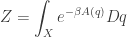
is its velocity. The partition function is then

where we integrate an exponential involving the action over the space of all paths 

There is a lot to say about this, but if we just want to get some answers, it’s best to sneak up on the problem gradually.
Discretizing time
We’ll start by treating time as discrete—a trick Feynman used in his original work. We’ll consider 


Let’s call the particle’s velocity between the (i-1)st and ith time steps


The action, defined as an integral, is now equal to a finite sum:

We’ll consider histories of the particle where its initial position is

but its final position 

and now we’re ready to apply the formulas we developed last time!
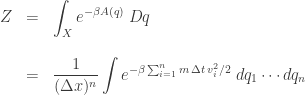
We saw last time that the partition function is the key to all wisdom, so let’s start with that. Naively, it’s
where

But there’s a subtlety here. Doing this integral requires a measure on our space of histories. Since the space of histories is just 


However, the partition function should be dimensionless! You can see why from the discussion of units last time. But the quantity 


I should however emphasize that despite the notation 
Now let’s compute the partition function. For starters, we have
Normally when I see an integral bristling with annoying constants like this, I switch to a system of units where most of them equal 1. But I’m trying to get a physical feel for quantropy, so I’ll leave them all in. That way, we can see how they affect the final answer.
Since
we can show that

To show this, we need to work out the Jacobian of the transformation from the 

We can rewrite the path integral using this change of variables:
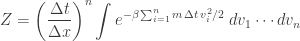
But since an exponential of a sum is a product of exponentials, this big fat n-tuple integral is really just a product of n ordinary integrals. And all these integrals are equal, so we just get some integral to the nth power! Let’s call the variable in this integral 

How do we do the integral here? Well, that’s easy…
Integrating Gaussians
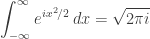
We should all know the integral of our favorite Gaussian. As a kid, my favorite was this:

because this looks the simplest. But now, I prefer this:
They’re both true, so why did my preference change? First, I now like 


Or course it doesn’t matter much: you just need to remember the integral of some Gaussian, or at least know how to calculate it. And you’ve probably read this quote:
A mathematician is someone to whom

is as obvious as 2+2=4 is to you and me. – Lord Kelvin
So, you probably learned the trick for doing this integral, so you can call yourself a mathematician.
Stretching the above Gaussian by a factor of 

This is clear when 
But this integral doesn’t converge if you slap absolute values on the function inside: in math jargon, the function inside isn’t ‘Lebesgue integrable’. But we can tame it in various ways. We can impose a ‘cutoff’ and then let it go to infinity:

or we can damp the oscillations, and then let the amount of damping go to zero:

We get the same answer either way, or indeed using many other methods. Since such tricks work for all the integrals I’ll write down, I won’t engage in further hand-wringing over this issue. We’ve got bigger things to worry about, like: what’s the physical meaning of quantropy?
Computing the partition function
Where were we? We had this formula for the partition function:

and now we’re letting ourselves use this formula:
even when

And a nice thing about keeping all these constants floating around is that we can use dimensional analysis to check our work. The partition function should be dimensionless, and it is! To see this, just remember that 

Expected action
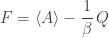
Now that we’ve got the partition function, what do we do with it? We can compute everything we care about. Remember, in statistical mechanics there’s a famous formula:
and last time we saw that similarly, in quantum mechanics we have:
where the classicality is

In other words:
Last time I showed you how to compute 

| Expected action | 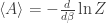 |
| Free action |  |
| Quantropy |  |
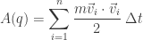
But let’s start with the expected action. The answer will be so amazingly simple, yet strange, that I’ll want to spend the rest of this post discussing it.
Using our hard-won formula

we get

Wow! When get an answer this simple, it must mean something! This formula is saying that the expected action of our freely moving quantum particle is proportional to 


Why don’t they matter? Well, you can see from the above calculation that they just disappear when we take the derivative of the logarithm containing them. That’s not a profound philosophical explanation, but it implies that our action could be any quadratic function like this:


where 

The numbers
The quadratic function we’re talking about here is an example of a quadratic form. Because the numbers
Whenever the action is a positive definite quadratic form on an n-dimensional vector space of histories, the expected action is

For example, take a free particle in 3d Euclidean space, and discretize time into
since now each velocity 

Poetically speaking,
So here’s a more intuitive way to think about our result:
In the path integral approach to quantum theory, each ‘decision’ made by the system contributes
There’s a lot more to say about this. For example, in the harmonic oscillator the action is a quadratic form, but it’s not positive definite. What happens then? But three more immediate questions leap to my mind:
1) Why is the expected action imaginary?
2) Should we worry that it diverges as 
3) Is this related to the heat capacity of an ideal gas?
So, let me conclude this post by trying to answer those.
Why is the expected action imaginary?
The action 
The reason is that we’re not taking its expected value with respect to an probability measure, but instead, with respect to a complex-valued measure. Last time we gave this very general definition:
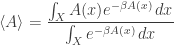
The action 
Later we’ll see a good reason why it has to be purely imaginary.
Why does it diverge as n → ∞?
Consider our particle on a line, with time discretized into
To take the continuum limit we must let 

That’s a bit sad, but not unexpected. It’s a lot like how the expected length of the path of a particle carrying out Brownian motion is infinite. In 3 dimensions, a typical Brownian path looks like this:

In fact the free quantum particle is just a ‘Wick-rotated’ version of Brownian motion, where we replace time by imaginary time, so the analogy is fairly close. The action we’re considering now is not exactly analogous to the arclength of a path:

Instead, it’s proportional to this quadratic form:

However, both these quantities diverge when we discretize Brownian motion and then take the continuum limit.
How sad should we be that the expected action is infinite in the continuum limit? Not too sad, I think. Any result that applies to all discretizations of a continuum problem should, I think, say something about that continuum problem. For us the expected action diverges, but the ‘expected action per decision’ is constant, and that’s something we can hope to understand even in the continuum limit!
Is this related to the heat capacity of an ideal gas?
That may seem like a strange question, unless you remember some formulas about the thermodynamics of an ideal gas!
Let’s say we’re in 3d Euclidean space. (Most of us already are, but some of my more spacy friends will need to pretend.) If we have an ideal gas made of 

where 
On the other hand, we’ve seen that in quantum mechanics, a single point particle will have an expected action of

after
These results look awfully similar. Are they related?
Yes! These are just two special cases of the same result! The energy of the ideal gas is a quadratic form on a

while in quantum mechanics we have

Mathematically, they are the exact same problem except that 
And this makes it even more obvious that the expected action must be imaginary… at least when the action is a positive definite quadratic form.


Very interesting article.
One thing about the n->inf limit, to me such limit seems unphysical.
In the case of brownian motion the fact that path length is infinite is a consequence of the point particle simplifying assumption, if we consider particles with definite size then a particle cannot change direction arbitrarily many times in any time frame because at some point the local neighborhood of the particle in question will be saturated with particles trying to pass momentum to it and such crowding effects will take over.
Analogously in the quantum case I believe there have to be physical reasons which place limits on how fast a particle can change it’s momentum. There has to be an energy scale which sets the limit, is there some known physics that could set such limit?
Personally I can imagine a scenario where the chaotic motions of particles that are taken into account by path integral formulation are not their intrinsic property but rather a cumulative effect of the background fields associated with all the other particles in either it’s local neighborhood or possibly the whole Universe. In such a picture the energy of the most energetic particle/field in the whole Universe would be a natural cut off scale, sure it could be large but not infinite.
As well you should, but the really fundamental constant is . This is the period of the exponential function, which is more fundamental than the cosine function. It shows up all over the place in very basic results, such as the Cauchy integral formula, roots of unity, etc. To be sure,
  also appears quite often, especially in applications where everything is (or can be) real, since it’s the magnitude of the fundamental
  . In college, we came up with a bunch of barred symbols (in homage to
  ), so we called
  ‘pi-bar’ (
 , if that shows up).
I forgot some ‘latex’s, and the strikethrough did not show up.
I fixed what I could easily fix.
As we’ve seen here, the partition function of the time-discretized free particle is
so you get to have your or your
  , whichever you want, but not both… which suggests that
  could be an interesting constant in its own right.
As you surely know, but others may not, is now called
  , because it represents one ‘turn’, and because
  looks like
  but twice as simple.
I don’t know if this was another mistake of mine or if it came it when John fixed my mistakes, but it’s that we called pi-bar.
John wrote:
I remember the surprised looks of my fellow students when I told them about this, so here is the explanation: The Lesbegue measure on the reals is translationally invariant and finite for a finite interval.
In an infinite dimensional separable Hilbert space a “Lesbegue measure” with these properties would have to assign a finite number to the unit ball (radius 1), and a finite number to the ball with radius, say, 1/10. The problem with this is that you can fit infinite many balls with radius 1/10 inside the unit ball, by positioning one at where
where  is the nth element of an orthonormal basis. Since the “Lesbegue measure” should be invariant for translations, it would have to assign each of these balls the same finite number as the one centered around the origin.
Thanks for explaining that. This fact played a huge role in my early life, when I was working with Segal on integrals over infinite-dimensional Hilbert spaces. Lebesgue measure is gone… but Gaussian measures (and ‘generalized measures’) still exist!
Very nice example. Especially your formula for the expected action. Congratulation for that.
What is next? Things diverge. That does not come unexpected. My initial response (cf. my last comment) to that situation was to restrict the domain for the paths from continuous functions to more regular things like bounded variation, or even
  . Since the expected action is somehow the arclength the integrals might converge then. However, such an approach seems to destroy the guiding analogy between statistical mechanics and what you are doing. Does it? After all, Brownian motion is highly irregular and nevertheless connected (by a ‘Wick-rotation’) to heat diffusion which is probably the most regular motion there is. It might even be possible to find some ‘natural’ space of paths.
Such or similar were my initial thoughts. After I read your article, in particular the part your discussion of the ideal gas, it occurred to me that there might be a less technical way to proceed. Roughly speaking, it might not be necessary to consider the case. What does (can) that mean? In the case of the ideal gas we are only interested in the energy of a huge number of particles, but not for infinitely many of them. Maybe, the analogue of ‘energy of
  particles in an ideal gas’ is not the time evolution of something, but ‘expected action of a particle running through
  gates’. I am not overly precise what I mean by a gate now. Just that it is in principle possible to have a huge number (
 ) of them in series and a particle passing them by ‘making decisions’. While in principle it is possible to let the number of gates run to infinity we are not interested in doing that since ‘reality’ limits the number of gates as it limits the number of particles in an ideal gas. Too weird? OK, I stop here.
In any case you have all tools at hand to introduce a potential and discuss the difficulties that come along.
Thanks for your comments! Maybe there’s a nice continuum limit of the expected action of a particle running through gates, meaning that we don’t take
  , but define a function of the particle’s positions at
  chosen times, namely the least possible action for a path going through those points at those times, and then compute its expected value using a real-time path integral. We’d need to introduce a time discretization and then show the limit exists as we remove this discretization. This is definitely true for the free particle, but that’s a specially easy case.
Anyway, I think some creative ideas are needed here…
Since Uwe said “gate”, I’m inclined to wonder what happens to the expected action of the particle with time in steps, if we observe the position at step
  ?
?
or… that’s what you already said, isn’t it?
In my mind, the n gates or signposts that are erected in the specification of the particle’s positions are strongly reminiscent of “collapse events.” By increasing n, we increase the finesse with which we specify what the particle can do on its way from point A to point B, and we make our description of the particle’s time evolution “more classical” – more like a trajectory and less like wavefunction evolution.
This increase in information content seems to require an increase in the action, relative to a fundamental unit, i hbar.
The connection to heat capacity is very interesting. Heat capacity is a key quantity in thermal physics, and I would hope to see it make it into the table of analogues!
To a physical chemist, the heat capacity measures how many joules of energy are required to cause a kelvin of temperature change. It is an extensive quantity, and, in my mind anyway, is a measure of “thermally accessible degrees of freedom.” Is this usefully related to the finesse with which we can (or have to) specify microscopic details of a macroscopically defined, thermal system?
The definition of (constant volume) heat capacity involves a derivative of internal energy with respect to temperature. The analogue on the quantum side would seem to involve a derivative of action with respect to i hbar.
This analogue might raise and answer (admittedly vague) questions like “quantitatively, how much more quantum would this system behave if i hbar were bigger?”
One final comment regarding the n “gates”: A study of the harmonic oscillator might be illuminating. In quantum optics it is possible to produce “squeezed states” of a cavity mode by coupling it resonantly to a detector at multiples of a resonance frequency. I wonder if judicious selection of the time schedule of selected gate points changes quantities like expected action, etc., in an understandable way.
The nice simple expected action looks like it maybe comes from the free particle being classical, so that doesn’t involve
  (i.e.
(i.e.  ). Does anything change if a quantum free particle is used instead?
I’m working with the quantum free particle; all the calculations here are quantum-theoretic. In the path integral approach to quantum mechanics, the action never involves Planck’s constant. Planck’s constant shows up in integrals over the space of paths, e.g. the partition function itself:
The expected action works out simply in this problem because the action is a quadratic function of the path
Linear or quadratic actions give exactly solvable theories and typically serve as the starting-point for further investigations. For example, the free particle and harmonic oscillator have quadratic actions. So, the expected action should also be easy to compute exactly for the harmonic oscillator. Particles in more complicated potentials will get a lot harder.
Consider the action
Being just a mathematician I can’t judge whether that is a physically realistic action. I think we have used that in school as a local approximation of gravity. Anyway, using all your assumptions (e.g. , the Gaussian integral aso.) the expected action can be computed as
For this is consistent with your result. The sum over
  can be evaluated explicitly and since
  is
is  the behaviour of the expected action is like
  .
.
Wow – you’re just a mathematician? You look like you know what you’re doing!
I’ve really been appreciating your comments in this quantropy discussion—you’re the only one brave enough to join in and actually do some calculations.
As you suspect, the action you wrote down describes a particle in a potential
which describes a constant force
So, if you’re doing experiments dropping neutrons and seeing how their wavefunctions spread out, this is the right action to use—at least until the neutron hits the floor and bounces!
• C. Codau, V.V. Nesvizhevsky, M. Fertl, G. Pignol and K.V. Protasov, Transitions between levels of a quantum bouncer induced by a noise-like perturbation.
But anyway, that’s a digression…
Any Lagrangian that’s a quadratic function of and
and  should be manageable, but some are easier than others. I did the very easiest one, and yours looks very nice too. I hadn’t thought of trying it, but it’s important because a constant force field is a simple approximate model for any force. I’d been wanting to do the harmonic oscillator, which should have its own charms.
A quantum bouncer. Interesting.
On the harmonic oscillator I can offer support albeit it might take a couple of days to find some spare time. So, if someone jumps in I would not be too disappointed.
Arghh! Don’t tell everybody! But honestly, so far I have no idea what quantropy actually means. Do you consider it possible that by extremizing quantropy 1) in the end one only gets garbage 2) one gets an alternative way to explain some known physics 3) one gets new effects. What would be the best possible outcome one could hope for ? … or is it too early to pose such questions ? What about a more ‘philosophical’ background article without formulas to get more people into it.
Uwe wrote:
Neither do I. That’s why I’m doing all these @*#$& calculations.
It’s not too early to pose them. It may be too early to answer them.
I’ve explained all the philosophical background I know, especially here and here. I don’t really want more people to get into the subject until I figure out the easy fun stuff myself. If I were a normal physicist I’d keep all these ideas secret until I published a paper or two.
But I’ll just repeat:
There’s a beautiful and precise 2 × 2 analogy square:
In three out of the four entries, we can derive everything starting from a minimum or maximum principle:
So, it seems insane for the fourth not to work the same way. We can figure out what quantum mechanics ‘extremizes’, and it’s quantropy. However, it’s complex-valued so we should really speak of a stationary principle rather than a minimum or maximum principle. And if you think harder you see that’s true in some of the other cases too. So we can say:
Now, it could turn out that the principle of stationary quantropy is just a mirage due to the divergences we’re seeing. Or, maybe it’s fine but only if we treat time as discrete: that would be quite interesting. It could be that we can only use it to derive results that can be derived in other ways. That’s also true about the principle of least action to some extent—Feynman tells how as a young student he was very big on doing everything with just , which is pretty ironic given his later work on path integrals. Or, it could be that the principle of stationary quantropy will give really new insights. That’s also true about the principle of least action.
But for now I (or we) just gotta think and calculate.
Maybe you should do this indeed. It would be less fun though.
You are not alone :-) For the action of the harmonic oscillator
the quantropic partition function is
Observe that for it is the partition function for the free particle. At least. The expected action is still linear in
  and does not depend on
The calculations are elementary and actually rather boring. In case you are interested in them I could dump them here or in my blog or private mail them. Whatever.
Uwe wrote:
Right. I have to strike a balance between caution and having fun. Since I have tenure, I can afford to have more fun. But I still like to be the first to publish stuff.
I figure that as long as most people think quantropy is a weird, stupid or useless idea, it’s safe for me to talk about it publicly. But I don’t want to recruit a lot of people into working on it before I’ve put something on the arXiv.
Thanks—but I’ll probably do them myself someday. I find I learn a lot from doing these calculations, even if in some sense they’re elementary and boring. They make me think about lots of things, in a way that reading a calculation does not. But being able to check whether my answer matches yours will be very nice, since I make lots of mistakes. So thanks for that!
Good! But what matters is not just that. What matters is the precise coefficient! And from your results we see the expected action is
And that’s great!
Let me explain why:
Since the expected action for the free particle is so simple, I’ve decided that the expected action is what I should focus on for now.
As I hinted in this blog post, in statistical mechanics, people make an enormous amount of fuss over the fact that
Strictly speaking this is only true for classical systems whose energy is a positive definite quadratic form on some finite-dimensional vector space. The ‘number of degrees of freedom’ is the dimension of that vector space. But since every smooth function can be approximated by a quadratic function near a nondegenerate minimum, this is approximately true for a vast number of classical systems.
In fact, you’ll often see this formula mistakenly used as a definition of temperature!
In my post, I noticed that for systems where the action is a positive definite quadratic form on a finite-dimensional vector space,
This is the precise analogue of what we know about statistical mechanics!
For the harmonic oscillator the action is still a quadratic form, but it’s not positive definite, so some new subtleties intrude. Nonetheless I expected the above principle would still hold, and you’re telling me it does.
These are some substantial objections against quantropy and once you elevate this from blog to arXiv you maybe want to deal with them. Thus it might be helpful for you to know why I do not think that this is useless (thereby giving some possible uses).
A sole analogy possibly won’t convince people. There is just not enough innovation and probably not a lot of physics and certainly no relevant mathematics contained. Such or similar might be a first opinion when dealing with this. Things change, at least for me, with the introduction of quantropy. Why is this the case? Now one can break the symmetry and introduce something new by making the integrals converge. For example, if you consider particles travelling along the paths with the speed of light you will eventually get a cutoff in the integrals. You have mentioned a cutoff in one of your articles as a way to define things. In this case the purely mathematical will be replaced by a physically hopefully more tractable velocity
  . Is such a computation new? Most likely not. Feynman an his follow ups could certainly do these computations. However, there is a slim chance that they simply were not interested in it for two reasons: Their integrals converged anyway and the resulting Schrödinger equation would contain an unwanted velocity parameter. The situation in the quantropy business is different. Here, a choice _has_ to be made since otherwise nothing converges. If it is the above choice of a “speed limit” reevaluating your motivating example for quantropy might lead to what you have called a “Feynman’s sum over histories formulation of quantum mechanics” augmented with a velocity parameter. My knowledge of physics is slim enough to consider this to be interesting.
With this thoughts I certainly do not want to diminish other choices to make the integrals converge or even robust approaches that do not consider convergence at all. Anything goes. These are just my (naive?) thoughts why one should not immediately discard this idea.
Uwe wrote:
What are you talking about, exactly, when you say ‘a sole analogy’?
At first I thought you meant the analogy between entropy and quantropy, but the last sentence suggest otherwise. The analogy between quantum mechanics and statistical mechanics? This analogy is already very famous, and there’s a huge amount of physics and mathematics in it. Many books have been written based on this analogy: for example, Glimm and Jaffe’s Quantum Physics: A Functional Integral Point of View constructs quantum field theories using Wick rotation to transform path integrals into statistical mechanics problems, and Barry Simon’s Functional Integration and Quantum Physics covers different aspects of the same territory. The subject of conformal field theory is another example: thanks to this analogy it leads a double life, on the one hand allowing people to understand critical points in 2d statistical mechanics problems, and on the quantum side playing a fundamental role in string theory.
So the first interesting thing about quantropy is that it’s an obvious yet apparently largely unexplored aspect of this already famous analogy.
The expression for the expected action makes me think of the expected energy of a quantum harmonic oscillator (and hence QFT). So by analogy maybe one could think of 1/2i * h/2pi as the eigenvalue of the ‘action operator’ and when n steps (for the 1D case) are taken it means n quanta of action (=’actons’?) are emitted just like n photons with energy h nu are absorbed/emitted when an electron moves to its nth eigenstate/drops down to the ground state.
Hmm! I’ve been thinking about strange things like this myself recently: the analogies between classical mechanics, thermodynamics, statistical mechanics and quantum mechanics lead to some strange possibilities like quantizing thermodynamics, quantizing quantum mechanics, etc. Of course ‘second quantization’ is a known thing, and known to be useful… but there could be other things, not yet explored, which are logically consistent and (who knows?) perhaps even useful somehow.
You’re right: the formula
for the ground state energy of the quantum harmonic oscillator looks suspiciously similar to the formula
for the ‘expected action per decision’ of a free quantum particle. But I don’t see a mathematical relationship underlying this similarity, so I’m reluctant to plunge in and try stuff!
On the other hand, there’s a clear mathematical relationship between
as the ‘expected action per decision’ for a free quantum particle and
as the ‘expected energy per degree of freedom’ for a classical harmonic oscillator.
That’s what I worked out in this post.
So, you (or someone) could try to find a precise mathematical relation between the
ground state energy of the quantum harmonic oscillator and the
expected action per degree of freedom of the classical harmonic oscillator. But the first number shows up as an eigenvalue of a differential operator, while the second shows up as the value of an integral (as in this post). Also, the first depends on the frequency of the oscillator, while the second does not! So I don’t see a connection.
Hi there
I’ve recently come across this series of posts and found them quite intriguing. I’ve often wondered if there might be a way to get to quantum theory by modifying classical (Bayesian) probability theory in some principled way, and this looks like it might be the beginning of a path that could lead in that direction.
It’s very interesting stuff, but there’s a slight conceptual issue that’s been bothering me, and I wonder whether thinking about it more might shed some more light on what this analogy really means. I hope I can express it clearly enough.
In the thermal case, when you derive the Boltzmann distribution by maximising the entropy, it’s done subject to to a constraint on the expected energy, i.e. you set , for some prescribed value
  . Once you’ve done the whole Lagrange multiplier thing you then have to choose the particular value for
  such that the constraint
  is satisfied.
  thus becomes a function of
  .
.
But then it turns out that in practice you often know and not
  , because the system is in contact with a heat bath that fixes the temperature. In this case you still get
  as a function of
  , but you plug in the value of
  to find
  and not the other way around.
Now, in your quantropy analogy you’re doing the latter thing. That is, you’re not finding a stationary point of the quantropy subject to a constraint for some particular known value of
  and then choosing
  such that the constraint is satisfied. Instead it looks like you’re using the Lagrange multiplier technique to find a functional relationship between
  and
and  and then plugging in a known value of
  (equal to
  ) to find
  .
.
So I’m wondering what that really means. I realise you probably don’t have an answer to that yourself, but it seems to me that thinking about it might (or might not) be a useful next step to take. Naively, it looks like it’s saying the universe is in contact with a sort of Wick-rotated heat bath with an imaginary temperature of . But I wonder if there’s some other, more sensible interpretation of this step.
I’m glad you liked these posts, Nathaniel! You wrote:
I don’t think of these as significantly different things. The way it always works when you’re looking for a stationary point of a function $f$ subject to a constraint on some other function $g$ is that you set
and solve the resulting equations. In this process, it’s pretty much always easier to pick a value of and find out what value the constraint
  than takes, rather than the other way around—though in terms of the original problem, you usually want to think of things the other way around.
In particular, I don’t see anything about the math of quantropy that differs from the math of entropy in this respect.
I agree, the math is exactly the same – it’s the interpretation I’m trying to get at. It’s kind of a subtle point, and I was afraid I wouldn’t be able to get it across clearly.
The point is that, when doing classical MaxEnt (which I do a lot), sometimes you know and want to work out
  , and sometimes you know
  and want to work out
  . I was just pointing out that for quantropy it’s always the latter case. $\lambda$ isn’t a variable whose value depends on the system’s state like $\beta$ is, but rather it is (or appears to be) a universal constant. Beyond that, my point isn’t really anything more than “hey, that’s interesting, I wonder what it means?”
To put it another way, if we lived in an isothermal universe (i.e. one where everything everywhere was connected to a heat bath at a constant temperature) then $\beta$ would have the same value for all systems, and so we’d think of it as a universal constant. That isn’t the universe we live in, though, and $\beta$ has different values for different systems. But for the quantropy case, $\lambda$ does seem to always have the same value, for every system, unless I’ve misunderstood something. That’s what I meant when I said it looks, naively, like the universe is in contact with a sort of Wick-rotated heat bath (or rather an action bath) with a constant imaginary temperature. I’m not saying that’s a plausible physical picture, just that it’s interesting that that’s what the maths seems to look like.
Interesting series of posts! Just a small typo at the end:
The last equation should obviously be
Glad you liked the posts! Actually Planck’s constant is analogous to inverse temperature, not temperature. To see this in an intuitive way, note that increasing Planck’s constant increases quantum fluctuations, while increasing temperature increases thermal fluctuations. Also: we get classical dynamics obeying the principle of least action when Planck’s constant goes to zero, while we get classical statics obeying the principle of least energy when the temperature goes to zero.
If you have carefully read all my previous posts on quantropy (Part 1, Part 2 and Part 3), there’s only a little new stuff here. But still, it’s better organized […]