We’re trying to get a little insight into the Earth’s glacial cycles, using very simple models. We have a long way to go, but let’s review where we are.
In Part 5 and Part 6, we studied a model where the Earth can be bistable. In other words, if the parameters are set right it has two stable states: one where it’s cold and stays cold because it’s icy and reflects lots of sunlight, and another where it’s hot and stays hot because it’s dark and absorbs lots of sunlight.
In Part 7 we saw a bistable system being pushed around by noise and also an oscillating ‘force’. When the parameters are set right, we see stochastic resonance: the noise amplifies the system’s response to the oscillations! This is supposed to remind us of how the Milankovich cycles in the Earth’s orbit may get amplified to cause glacial cycles. But this system was not based on any model of the Earth’s climate.
Now a student in this course has put the pieces together! Try this program by Michael Knap and see what happens:
• A stochastic energy balance model.
Remember, our simple model of the Earth’s climate amounted to this differential equation:
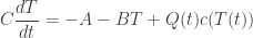
Here:
• 


• 
• 

Here 


Or, you can choose

where 
• 

Here 


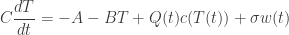
Now Michael Knap is adding noise, giving this equation:
where 


where 

Play around with Michael’s model and see what effects you can get!
Puzzle. List some of the main reasons this model is not yet ready for realistic investigations of how the Milankovitch cycles cause glacial cycles.
You can think of some big reasons just knowing what I’ve told you already in this course. But you’ll be able to think of some more once you know more about Milankovitch cycles.
Milankovitch cycles
We’ve been having fun with models, and we’ve been learning something from them, but now it’s time to go back and think harder about what’s really going on.
As I keep hinting, a lot of scientists believe that the Earth’s glacial cycles are related to cyclic changes in the Earth’s orbit and the tilt of its axis. Since one of the first scientists to carefully study this issue was Milutin Milankovitch, these are called Milankovitch cycles. Now let’s look at them in more detail.
The three major types of Milankovitch cycle are:
• changes in the eccentricity of the Earth’s orbit – that is, how much the orbit deviates from being a circle:

(changes greatly exaggerated)
• changes in the obliquity, or tilt of the Earth’s axis:

• precession, meaning changes in the direction of the Earth’s axis relative to the fixed stars:

The first important thing to realize is this: it’s not obvious that Milankovitch cycles can cause glacial cycles. During a glacial period, the Earth is about 5°C cooler than it is now. But the Milankovitch cycles barely affect the overall annual amount of solar radiation hitting the Earth!
This fact is clear for precession or changes in obliquity, since these just involve the tilt of the Earth’s axis, and the Earth is nearly a sphere. The amount of Sun hitting a sphere doesn’t depend on how the sphere is ’tilted’.
For changes in the eccentricity of the Earth’s orbit, this fact is a bit less obvious. After all, when the orbit is more eccentric, the Earth gets closer to the Sun sometimes, but farther at other times. So you need to actually sit down and do some math to figure out the net effect. Luckily, Greg Egan did this calculation in a very nice way, earlier here on the Azimuth blog. I’ll show you his calculation at the end of this article. It turns out that when the Earth’s orbit is at its most eccentric, it gets very, very slightly more energy from the Sun each year: 0.167% more than when its orbit is at its least eccentric. This is not enough to warm the Earth very much.
So, there are interesting puzzles involved in the Milankovitch cycles. They don’t affect the total amount of radiation that hits the Earth each year—not much, anyway—but they do cause substantial changes in the amount of radiation that hits the Earth at various different latitudes in various different seasons. We need to understand what such changes might do.
James Croll was one of the first to think about this, back around 1875. He decided that what really matters is the amount of sunlight hitting the far northern latitudes in winter. When this was low, he claimed, glaciers would tend to form and an ice age would start. But later, in the 1920s, Milankovitch made the opposite claim: what really matters is the amount of sunlight hitting the far northern latitudes in summer. When this was low, an ice age would start.
If we take a quick look at the data, we see that the truth is not obvious:

I like this graph because it’s pretty… but I wish the vertical axes were labelled. We will see some more precise graphs in future weeks.
Nonetheless, this graph gives some idea of what’s going on. Precession, obliquity and eccentricity vary in complex but still predictable ways. From this you can compute the amount of solar energy that hits the surface of the Earth’s atmosphere on July 1st at a latitude of 65° N. That’s the yellow curve. People believe this quantity has some relation to the Earth’s temperature, as shown by the black curve at bottom. However, the relation is far from clear!
Indeed, if you only look at this graph, you might easily decide that Milankovitch cycles are not important in causing glacial cycles. But people have analyzed temperature proxies over long spans of time, and found evidence for cyclic changes at periods that match those of the Milankovitch cycles. Here’s a classic paper on this subject:
• J. D. Hays, J. Imbrie, and N. J. Shackleton, Variations in the earth’s orbit: pacemaker of the Ice Ages, Science 194 (1976), 1121-1132.
They selected two sediment cores from the Indian ocean, which contain sediments deposited over the last 450,000 years. They measured:
1) Ts, an estimate of summer sea-surface temperatures at the core site, derived from a statistical analysis of tiny organisms called radiolarians found in the sediments.
2) δ18O, the excess of the heavy isotope of oxygen in tiny organisms called foraminifera also found in the sediments.
3) The percentage of radiolarians that are Cycladophora davisiana—a certain species not used in the estimation of Ts.
Identical samples were analyzed for the three variables at 10-centimeter intervals throughout each core. Then they took a Fourier transform of this data to see at which frequencies these variables wiggle the most! When we take the Fourier transform of a function and then square it, the result is called the power spectrum. So, they actually graphed the power spectra for these three variables:
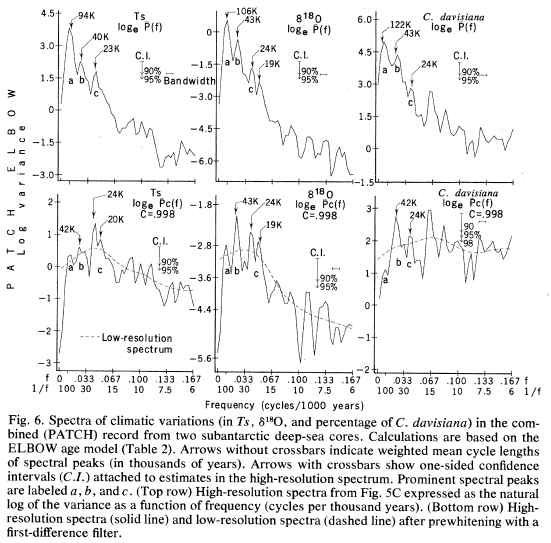
The top graph shows the power spectra for Ts, δ18O, and the percentage of Cycladophora davisiana. The second one shows the spectra after a bit of extra messing around. Either way, there seem to be peaks at frequencies of 19, 23, 42 and roughly 100 thousand years. However the last number is quite fuzzy: if you look, you’ll see the three different power spectra have peaks at 94, 106 and 122 thousand years.
So, some sort of cycles seem to be occurring. This is far from the only piece of evidence, but it’s a famous one.
Now let’s go over the three major forms of Milankovitch cycle, and keep our eye out for cycles that take place every 19, 23, 42 or roughly 100 thousand years!
Eccentricity
The Earth’s orbit is an ellipse, and the eccentricity of this ellipse says how far it is from being circular. But the eccentricity of the Earth’s orbit slowly changes: it varies from being nearly circular, with an eccentricity of 0.005, to being more strongly elliptical, with an eccentricity of 0.058. The mean eccentricity is 0.028. There are several periodic components to these variations. The strongest occurs with a period of 413,000 years, and changes the eccentricity by ±0.012. Two other components have periods of 95,000 and 123,000 years.
The eccentricity affects the percentage difference in incoming solar radiation between the perihelion, the point where the Earth is closest to the Sun, and the aphelion, when it is farthest from the Sun. This works as follows. The percentage difference between the Earth’s distance from the Sun at perihelion and aphelion is twice the eccentricity, and the percentage change in incoming solar radiation is about twice that. The first fact follows from the definition of eccentricity, while the second follows from differentiating the inverse-square relationship between brightness and distance.
Right now the eccentricity is 0.0167, or 1.67%. Thus, the distance from the Earth to Sun varies 3.34% over the course of a year. This in turn gives an annual variation in incoming solar radiation of about 6.68%. Note that this is not the cause of the seasons: those arise due to the Earth’s tilt, and occur at different times in the northern and southern hemispheres.
Obliquity
The angle of the Earth’s axial tilt with respect to the plane of its orbit, called the obliquity, varies between 22.1° and 24.5° in a roughly periodic way, with a period of 41,000 years. When the obliquity is high, the strength of seasonal variations is stronger.
Right now the obliquity is 23.44°, roughly halfway between its extreme values. It is decreasing, and will reach its minimum value around the year 10,000 CE.
Precession
The slow turning in the direction of the Earth’s axis of rotation relative to the fixed stars, called precession, has a period of roughly 23,000 years. As precession occurs, the seasons drift in and out of phase with the perihelion and aphelion of the Earth’s orbit.
Right now the perihelion occurs during the southern hemisphere’s summer, while the aphelion is reached during the southern winter. This tends to make the southern hemisphere seasons more extreme than the northern hemisphere seasons.
The gradual precession of the Earth is not due to the same physical mechanism as the wobbling of the top. That sort of wobbling does occur, but it has a period of only 427 days. The 23,000-year precession is due to tidal interactions between the Earth, Sun and Moon. For details, see:
• John Baez, The wobbling of the Earth and other curiosities.
In the real world, most things get more complicated the more carefully you look at them. For example, precession actually has several periodic components. According to André Berger, a top expert on changes in the Earth’s orbit, the four biggest components have these periods:
• 23,700 years
• 22,400 years
• 18,980 years
• 19,160 years
in order of decreasing strength. But in geology, these tend to show up either as a single peak around the mean value of 21,000 years, or two peaks at frequencies of 23,000 and 19,000 years.
To add to the fun, the three effects I’ve listed—changes in eccentricity, changes in obliquity, and precession—are not independent. According to Berger, cycles in eccentricity arise from ‘beats’ between different precession cycles:
• The 95,000-year eccentricity cycle arises from a beat between the 23,700-year and 19,000-year precession cycles.
• The 123,000-year eccentricity cycle arises from a beat between the 22,4000-year and 18,000-year precession cycles.
I’d like to delve into all this stuff more deeply someday, but I haven’t had time yet. For now, let me just refer you to this classic review paper:
• André Berger, Pleistocene climatic variability at astronomical frequencies, Quaternary International 2 (1989), 1-14.
Later, as I get up to speed, I’ll talk about more modern work.
Paleontology versus astronomy
Now we can compare the data from ocean sediments to the Milankovitch cycles as computed in astronomy:
• The roughly 19,000-year cycle in ocean sediments may come from 18,980-year and 19,160-year precession cycles.
• The roughly 23,000-year cycle in ocean sediments may come from 23,700-year precession cycle.
• The roughly 42,000-year cycle in ocean sediments may come from the 41,000-year obliquity cycle.
• The roughly 100,000-year cycle in ocean sediments may come from the 95,000-year and 123,000-year eccentricity cycles.
Again, the last one looks the most fuzzy. As we saw, different kinds of sediments seem to indicate cycles of 94, 106 and 122 thousand years. At least two of these periods match eccentricity cycles fairly well. But a detailed analysis would be required to distinguish between real effects and coincidences in this subject! Such analyses have been done, of course. But until I study them more, I won’t try to discuss them.


“As the eccentricity of the Earth’s orbit changes, the orbital period T, and hence the semi-major axis a, remains almost constant.”
Why does T remain almost constant? And related: why does the eccentricity change?
I imagine the answer to the latter is interactions with other planets. Why would such interactions leave periods unchanged?
Graham, the orbital period and semi-major axis remain very nearly constant because the orbital energy of the earth remains very nearly constant. That is, the earth is not spiraling in to the sun or out from it. (Of course over really long time that’s not true as the sun’s mass changes, but never mind.)
Yes, eccentricity changes are a result of interactions with other planets (mostly Jupiter). Small (relative to the total!) amounts of angular momentum are exchanged in a cycle. If enough energy was exchanged to alter the orbital period, then something dramatic (like ejection) would likely occur. So chalk it up to the strong anthropic principle – the resonances are small, stable, and mostly angular momentum rather than energy, because we’re here to observe them.
Thanks GFW, but your explanation does not satisfy me.
You say “the orbital energy of the earth remains very nearly constant.” and “amounts of angular momentum are exchanged in a cycle.” But changing angular momentum, that is, J, in John’s notation means a proportional change in the period T (doesn’t it?). But John (and Greg) are assuming T does not change. You can have constant energy E or constant T but not both (as fas as I can see), and somebody needs to decide which one is going to be asumed and say why it is assumed.
Also, I don’t see why you couldn’t have energy exchanged between orbits in a way that is not chaotic, and does not spiral out of control. The energy might flow one way during part of the cycle and back again during the rest.
I need to learn why T doesn’t change. I’ve been assured this is the case in papers by the supposed experts in the subject, and it seems plausible, but I don’t understand it well enough. Wikipedia gives a whopping big clue which matches my own guess:
It gives this reference:
• A. Berger, M. F. Loutre and J. L. Mélice, Equatorial insolation: from precession harmonics to eccentricity frequencies, Clim. Past Discuss. 2 (2006), 519–533.
Hmm, this doesn’t seem to explain the issue at hand, but it’s an interesting paper nonetheless!
A “Sun >> Jupiter >> Earth” model shouldn’t be too hard…
The Wikipedia article says that the semi-major axis is an ‘adiabatic invariant’. This suggests that it remains unchanged, not just by certain special perturbations, but all perturbations. It might be easier to prove this than to solve any particular 3-body problem!
The theme of adiabatic invariants is important in physics, and as you’ll see if you click that link, the area in phase space enclosed by an orbit is an adiabatic invariant that played a big role in the early history of quantum mechanics. So, I’m hoping that for elliptical orbits in a 1/r2 force law the semi-major axis is a function of this quantity.
Okay… so I have my work cut out for me, though probably I’ll take the lazy route and grab a book on perturbation theory in celestial mechanics.
I only stumbled on this question four years later, but since it reflects some misconceptions about the relationships between the quantities involved …
… I thought it was worth trying to set the record straight on the same page.
If you fix the masses of two bodies orbiting under their mutual gravitational attraction, then the total energy (kinetic plus potential) , the semi-major axis of their orbit,
  , and the period of their orbit,
  , are all determined by specifying just one of these three quantities. For example, in terms of
  , we have:
where and
and  are the total mass and reduced mass of the two bodies, and for something like the Earth-Sun system are very close to being just the mass of the Sun and the mass of the Earth.
Contrary to the assumptions in the question, you can change the angular momentum of the system while holding the energy, semi-major axis and period of the orbit constant. We have:
where is the eccentricity.
So changes in angular momentum in an orbit of fixed energy (and hence fixed period and fixed semi-major axis) just correspond to changes in eccentricity. The period doesn’t need to change in order for the angular momentum to change; rather, the change in angular momentum arises from the change in the shape of the orbit.
Thanks! I’m thinking about other things right now, but it’s good to get this straightened out. You seem to be in a mood for thinking about orbital mechanics.
It’s good to see that you are finally getting it. Milankovitch cycles do not cause Ice Ages, but they do affect the timing of glaciation/inter-glaciation periods. The Milankovitch cycles are not something new that only appeared during the Pleistocene. They’ve been around for ten of millions of years, if not longer.
Please also take the time to also finally notice that globally averaged temperatures in the last 1000 years have varied +1,-2F despite constant CO2 levels of 280ppm. Note that during the last glaciation, CO2 levels were at 180ppm and globally averaged temperatures were -16F lower than they were today yet since then, CO2 levels have risen another astonishing 100ppm, yet temperatures have only risen a paltry 1.26F. We should have had a huge change in temperature according to all the “experts” in this matter. If I raised the temperature in your house by 1.26F, would you even be able to notice it? And yet the Earth is suddenly so ultra-sensitive to temperatures, that 1.26 is supposed to cause huge, dramatic changes in our weather systems? Are we talking magic or science here? It seems that there are a lot of people out there that talk like they can do the math but are unable to the math as it actually applies to reality.
Maybe this has something to do with CO2 levels *lagging* large temperature variations by an average of 800 years? Clearly, there are feedback mechanisms that vastly overwhelm CO2 effects. Why don’t you explore those feedback mechanisms?
“[The current anthropomorphic global warming nonsense is based on] inherently untrustworthy climate models, similar to those that cannot accurately forecast the weather a week from now”. (Dr. Richard Lindzen)
These “experts” can’t tell us what the weather is going to be like three days from now and we are supposed to believe them when they tell us what the weather is going to be like 100 years from now? It’s about politics, not science.
Have you already commented on the puzzle somewhere?
I gave a few answers in class, but I’m still hoping someone here will try to answer it!
What about effects of Earth’s geothermal energy on climate?
Perhaps those orbital cycles affect patterns of magma convection in the mantle through tidal effects as they alter which latitudes are closest to the Moon (if my understanding of them is correct). This could alter heat transfer to the surface and affect global climate.
Fascinating post, deserves much more time than I’ve given it so far. I do find one sentence puzzling:
“Indeed, if you only look at this graph, you might easily decide that Milankovitch cycles are not important in causing glacial cycles.”
My eyeballs tell me something very different. When I scan the precession curve I see exactly eleven regions of relatively high amplitude, at roughly 100kyr intervals. Coincident with each of these eleven regions (and nowhere else) I see a significant peak of the black temperature curve. (OK, two of the temperature peaks are double peaks, and the high-precession-amplitude regions at 400kyr and 800kry are decidedly wimpy, but they are also decidedly there, and despite these anomalies the overall pattern described fairly screams out at me).
Maybe my ancestors were the ones always issuing false-positive predator calls in the jungle (if so, belated apologies:-)
arch 1,
Wow, you and I wear different glasses. I see how precession is related to eccentricity, but two interglacials near 400 and 800kya occur at low eccentricity and low precession amplitude. It is interesting that Dr. Berger claims the “beat” of precession modulates eccentricity. Seems more likely the other way around. Precession isn’t beating on anything. The earth just passively sits at whatever angle dictated by obliquity and has inevitable phase relative to eccentricity such that different seasons pertain to aphelion.
I didn’t manage to cover everything I intended last time, so I’m moving the stuff about the eccentricity of the Earth’s orbit to this week […]
Didier Paillard wrote:
I’m not including reference numbers, but here he cites a famous paper which we discussed in Part 8:
• J. D. Hays, J. Imbrie, and N. J. Shackleton, Variations in the earth’s orbit: pacemaker of the Ice Ages, Science 194 (1976), 1121–1132.