This quarter my graduate seminar at UCR will be about network theory. I have a few students starting work on this, so it seems like a good chance to think harder about the foundations of the subject. I’ve decided that bicategories of spans play a basic role, so I want to talk about those.
If you haven’t read the series up to now, don’t worry! Nothing I do for a while will rely on that earlier stuff. I want a fresh start. But just for a minute, I want to talk about the big picture: how the new stuff will relate to the old stuff.
So far this series has been talking about three closely related kinds of networks:
• Markov processes
• stochastic Petri nets
• stochastic reaction networks
but there are many other kinds of networks, and I want to bring some more into play:
• circuit diagrams
• bond graphs
• signal-flow graphs
These come from the world of control theory and engineering—especially electrical engineering, but also mechanical, hydraulic and other kinds of engineering.
My goal is not to tour different formalisms, but to integrate them into a single framework, so we can easily take ideas and theorems from one discipline and apply them to another.
For example, in Part 16 we saw that a special class of Markov processes can also be seen as a special class of circuit diagrams: namely, electrical circuits made of resistors. Also, in Part 17 we saw that stochastic Petri nets and stochastic reaction networks are just two different ways of talking about the same thing. This allows us to take results from chemistry—where they like stochastic reaction networks, which they call ‘chemical reaction networks’—and apply them to epidemiology, where they like stochastic Petri nets, which they call ‘compartmental models’.
As you can see, fighting through the thicket of terminology is half the battle here! The problem is that people in different applied subjects keep reinventing the same mathematics, using terminologies specific to their own interests… making it harder to see how generally applicable their work actually is. But we can’t blame them for doing this. It’s the job of mathematicians to step in, learn all this stuff, and extract the general ideas.
We can see a similar thing happening when writing was invented in ancient Mesopotamia, around 3000 BC. Different trades invented their own numbering systems! A base-60 system, the S system, was used to count most discrete objects, such as sheep or people. But for ‘rations’ such as cheese or fish, they used a base 120 system, the B system. Another system, the ŠE system, was used to measure quantities of grain. There were about a dozen such systems! Only later did they get standardized.
Circuit diagrams
But enough chit-chat; let’s get to work. I want to talk about circuit diagrams—diagrams of electrical circuits. They can get really complicated:

This is a 10-watt audio amplifier with bass boost. It looks quite intimidating. But I’ll start with a simple class of circuit diagrams, made of just a few kinds of parts:
• resistors,
• inductors,
• capacitors,
• voltage sources
and maybe some others later on. I’ll explain how you can translate any such diagram into a system of differential equations that describes how the voltages and currents along the wires change with time.
This is something you’d learn in a basic course on electrical engineering, at least back in the old days before analogue circuits had been largely replaced by digital ones. But my goal is different. I’m not mainly interested in electrical circuits per se: to me the important thing is how circuit diagrams provide a pictorial way of reasoning about differential equations… and how we can use the differential equations to describe many kinds of systems, not just electrical circuits.
So, I won’t spend much time explaining why electrical circuits do what they do—see the links for that. I’ll focus on the math of circuit diagrams, and how they apply to many different subjects, not just electrical circuits.
Let’s start with an example:

This describes a current flowing around a loop of wire with 4 elements on it: a resistor, an inductor, a capacitor, and a voltage source—for example, a battery. Each of these elements is designated by a cute symbol, and each has a real number associated to it:
• This is a resistor:

and it comes with a number 
• This is an inductor:

and it comes with a number 
• This is a capacitor:

and it comes with a number 
• This is a voltage source:

and it comes with a number 
You may wonder why inductance got called 


Here’s another example:

This example has two new features. First, it has places where wires meet, drawn as black dots. These dots are often called nodes, or sometimes vertices. Since ‘vertex’ starts with V and so does ‘voltage’, let’s call the dots ‘nodes’. Roughly speaking, a graph is a thing with nodes and edges, like this:
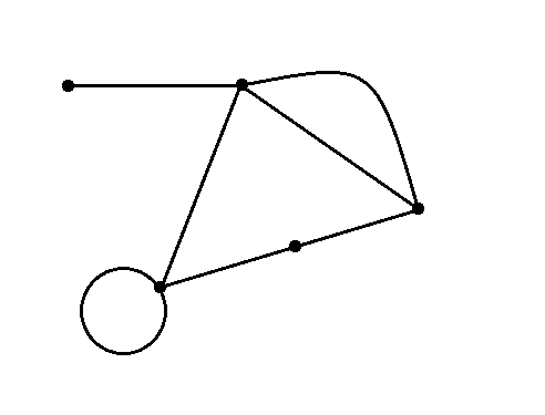
This suggests that in our circuit, the wires with elements on them should be seen as edges of a graph. Or perhaps just the wires should be seen as edges, and the elements should be seen as nodes! This is an example of a ‘design decision’ we have to make when formalizing the theory of circuit diagrams. There are also various different precise definitions of ‘graph’, and we need to try to choose the best one.
A second new feature of this example is that it has some white dots called terminals, where wires end. Mathematically these terminals are also nodes in our graph, but they play a special role: they are places where we are allowed to connect this circuit to another circuit. You’ll notice this circuit doesn’t have a voltage source. So, it’s like piece of electrical equipment without its own battery. We need to plug it in for it to do anything interesting!
This is very important. Big complicated electrical circuits are often made by hooking together smaller ones. The pieces are best thought of as ‘open systems’: that is, physical systems that interact with the outside world. Traditionally, a lot of physics focuses on ‘closed systems’, which don’t interact with the outside the world—the part of the world we aren’t modeling. But network theory is all about how we can connect open systems together to form larger open systems (or closed systems). And this is one place where category shows up. As we’ll see, we can think of an open system as a ‘morphism’ going from some inputs to some outputs, and we can ‘compose’ morphisms to get new morphisms by hooking them together.
Differential equations from circuit diagrams
Let me sketch how to get a bunch of ordinary differential equations from a circuit diagram. These equations will say what the circuit does.
We start with a graph having some set 


So, define a graph to consist of two functions

Then each edge 


(This kind of graph is often called a directed multigraph or quiver, to distinguish it from other kinds, but I’ll just say ‘graph’.)
Next, each edge is labelled by one of four elements: resistor, capacitor, inductor or voltage source. It’s also labelled by a real number, which we call the resistance, capacitance, inductance or voltage of that element. We will make this part prettier later on, so we can easily introduce more kinds of elements without any trouble.
Finally, we specify a subset 
Our goal now is to write down some ordinary differential equations that say how a bunch of variables change with time. These variables come in two kinds:
• Each edge 


• Each edge 

We now write down a bunch of equations obeyed by these currents and voltages. First there are some equations called Kirchhoff’s laws:
• Kirchhoff’s current law says that for each node that is not a terminal, the total current flowing into that node equals the total current flowing out. In other words:

for each node 
• Kirchhoff’s voltage law says that we can choose for each node a potential 

such that
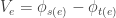
for each 
In addition to Kirchhoff’s laws, there’s an equation for each edge, relating the current and voltage on that edge. The details of this equation depends on the element labelling that edge, so we consider the four cases in turn:
• If our edge 
we write the equation

This is called Ohm’s law.
• If our edge
we write the equation

I don’t know a name for this equation, but you can read about it here.
• If our edge
we write the equation

I don’t know a name for this equation, but you can read about it here.
• If our edge 
we write the equation

This explains the term ‘voltage source’.
Puzzles
Next time we’ll look at some examples and see how we can start polishing up this formalism into something more pretty. But you can get to work now:
Puzzle 1. Starting from the rules above, write down and simplify the equations for this circuit:

Puzzle 2. Do the same for this circuit:

Puzzle 3. If we added a fifth kind of element, our rules for getting equations from circuit diagrams would have more symmetry between voltages and currents. What is this extra element?


You need a current source.
I am absolutely besotted with your idea of touring different formalisms. Please do let me know where I can buy this in book format, imho it would be something worth reading and rereading.
From my admittedly limited perspective, it also rather naturally leads to information theory and then to Kolmogorov complexity, and possibly to Dr. Stogatz’s work over at MIT.
Really looking forward to further posts. Thank you so much for sharing.
Thanks! I admit that I enjoy touring different formalisms, and it’s good to learn them, so we can talk to more people… but I also want to do some ‘data compression’, and reduce the number of required formalisms down to some bare minimum, and understand how they’re related.
Parts 2-26 of this network theory series will become a book fairly soon, and you can download a draft here. I’m not sure what I’ll do with the forthcoming parts yet. Maybe someday I’ll write a bigger, better book. But one book at a time!
Problem 1.
Apply Kirchhoff’s voltage law:
Take a time derivative:
The current is constant on the full loop. The dynamics of the components obey their own equations:
Therefore,
from which the time dependence of the three components can be found, given .
.
Great! And if we think of the current as the time derivative of something else—namely the charge on the capacitor’s plate:
then we can rewrite this as
which should remind us intensely of the equation describing the height of a particle of mass
  hanging on a massless spring with spring constant
  and damping coefficient
  , being pushed on by some force
  :
:
And this is part of the grand set of analogies people have developed between electrical circuits, mechanics, and many other subjects.
I recently found some nice stuff in electric circuits:
http://www.quantum-chemistry-history.com/Kron_Dat/Kron-1945/Kron-JAP-1945/Kron-JAP-1945.htm
These elaborate circuit equivalents were not only used as intellectual exercise, but as actual analog computers for solving differential equations, before digital computers.
Gerard
Thanks for the link! It’s nice to hear from you again! Of course I know your website:
• Gerard Westendorp, Electric circuit diagram equivalents of fields.
I’m interested in these things again: not using electric circuits as analogue computers, but using ideas in electric circuit theory to help develop a common category-theoretic formulation of many kinds of systems: first linear ones, and then nonlinear ones.
You can get an idea of what I mean from this book:
• Forbes T. Brown, Engineering System Dynamics: A Unified Graph-Centered Approach, CRC Press, 2007.
It’s huge (1078 pages, for only $131), very nice, but it uses bond graphs instead of electrical circuit diagrams. They’re roughly equivalent formalisms, and I’ll try to talk about both of them in this series.
Hi John,
Glad you still like my website, I needed a bit of pep talk. I’ve been a bit inactive on the web lately. I’ve been working on electric circuits, but unable to finalize it on the website yet, its kind of a tough chapter. It turns out there is a cool relation between (n+1)+1 dimensional space, Cayley-Menger matrices and electric circuits on triangulated grids. Related also to the Einstein equations, but as I said, progress is slow. But discussions like these might speed things up.
As an engineer, I have used electric circuits for thermal and acoustic applications. Especially the acoustics got me interested in electric circuits. For example, it is very convenient to model what happens acoustically when you drill a small hole somewhere in a long pipe, things like that. Maybe I should write a bit more on it, although there is a book by Beranek that is kind of a classic on the subject.
Looking foreward to more discussions on this. I am convinced the subject is by no means exhausted. I know bond graphs, but somehow I tend to prefer circuits.
Gerard
I’m not convinced that bond graphs are ‘better’, though the people who work deeply on these analogies seem to like them. I will try to state a mathematical theorem relating them to circuit diagrams in a precise way—that’s probably more important than deciding which one is ‘better’.
It seems to me that circuits are more general than bond graphs, since I do not know of a way to reperesent lattice shaped circuits into n-port networks and thus bond graphs
Yes, circuits are a bit more general than bond graphs, and that’s why I’m focusing on them here. Later I’ll describe a category where circuits are morphisms, and bond graphs will give an important subcategory.
Nice to see somebody interested in Kron. I am particularly interested in possible connections between Kron’s work & Information Geometry. I am fairly confident that the connection exists. Amai’s supervisor, Kazuo Kondo, was deeply influenced by Kron. Kondo’s research group, the RAAG, was largely dedicated to extending Kron’s geometrical idea’s. Amari’s master’s and doctoral theses were titled Topological and Information-Theoretical Foundation of Diakoptics and Codiakoptics. and Diakoptics of Information Spaces respectively, “diakoptics” being the term Kron coined for his methods. Unfortunately, my understanding of both Information Geometry and Diakoptics is currently too limited to say anything useful about the connection. However, I think it should help tie together a number of threads in this forum, particularly given that Kron, Kondo & the RAAG formulated much of their ideas in terms of tensor geometry.
‘Diakoptics’ sounds a bit weird, but the Wikipedia article on it says:
I’ve heard of the ‘method of tearing’ before in Jan Willems’ expository articles on control theory. I don’t really know how this method works, but one of my main concerns these days is how to use category theory to describe the process of building a physical system out of interacting parts. ‘Tearing’ sounds like the reverse operation. I can’t help but think it’s logically secondary. But I need to get a sense of how people use it in practice.
I think that the whole point of diakoptics/tearing is to solve the parts and then glue the solutions back together. So one tears systems, but glues solutions. This reminds me Joseph Goguen’s & Grant Malcolm’s work on modelling (de)composition of systems using sheaves in category theory. Malcolm also has interests in biological modelling and diagrams (the broad sense of the word, not just categories)
Another interesting aspect of Kron’s work is that when he treated moving systems like EM motors & generators using non linear coordinate transformations, making real use tensors and differential geometry.
Problem 2.
Here
and
since , therefore
and
Thanks! I think one fun thing to do with this problem is to work out the total current through the circuit:
in terms of the voltage across the two terminals,
in the case where the voltage varies sinusoidally with time, for example
for some frequency (Here I’m using complex voltages, which makes the math simpler.) We should see that this circuit acts as a band-pass filter. In other words, when
we should see that
solves the equations for some function , which we can work out. Moreover, we should see that
  biggest when
  is near a certain frequency, and smaller for frequencies far away from that. So, we can use this circuit to filter a signal, amplifying the part whose frequency is near this special frequency, and damping out the rest.
I haven’t actually done the calculation yet…
In this case you suggest,

We will define and we will find
  by summing the voltage around the loop with the resistor and inductor.
To solve the above, we can use an integrating factor, yeilding
Returning to the expression for the total current, and using
results in
the voltage appears in each term, so we weill consider the constant factor (John’s above
above
For the voltage and current to be in phase, the complex part of this expression must vanish. In other works,
I was curious to see what would happen using an extremization principle instead of assuming the voltage and current must be in phase. is marginally easier to deal with as
  than after the denominator is made real, so it was at that point that I diverged from your calculation.

 .
.
 .
.
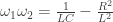
ends up having two pure imaginary solutions:
Their product is real, and looks somewhat familiar…
Hey ! Love your work.
In puzzle 3. are you talking about the memristor of Leon Chua ?
No, though I know why you’re saying that.
In the four elements I describe, there’s almost a symmetry which:
• interchanges voltage and current
• interchanges inductance and capacitance
• interchanges resistance and conductance
But to make this symmetry complete we need a fifth element.
By the way, there’s a movie about this puzzle.
Would you perhaps be summoning the fabled ‘current source’ from outer space to protect mankind from cosmic evil?
Thx for the explanation. I was thinking of the (constant) current source also but I couldn’t resist throwing in the idea of the memristor ha ha. It is a relatively new idea that opens fabulous technology in the years to come. I think that we should get used to see it around. In my opinion it should definitely belong to the picture.
The memristor also fits into the pictures, but it’s more subtle. I talked about it on week294 of This Week’s Finds. This was part of a series of articles that was sort of a warmup for this course.
I think this is a beautiful intro to electrical circuits.
In general if you have a graph of N edges you end up with 2N unknowns (currents and voltages along each edge), but you also have 2N equations (N equations for each component law, and N from the Kirchhoff rules), which allow you to actually solve the system of ODEs.
Regarding the “fifth element”, i think a current source ( ) is definitely needed for symmetry, but perhaps you mean something else.
Thanks!
As HK, David Lyon and you point out, we need a current source to be the symmetrical partner to the voltage source. It’s drawn like this, at least in the US:
The for current comes from “intensity of current”.
Oh, that’s interesting! Thanks!
Or to be really precise, from “intensité de courant” or just “intensité” which is what a certain André-Marie Ampère usually called it. The I seems to have stuck when his works were translated to English.
This may well be something you might be expanding on later in the course, but: both the Kirchoff laws are “linear”. (Eg, it’s the sum of the incoming currents that equals the outgoing currents whereas at least potentially one could imagine a rule that the sum of squares of incoming “flow” must equal the sum of squares of outgoing “flow”, say.) Obviously physical electricity turns out to work like that, but is there a more abstract reason for that the key rules are “linear” and that things don’t work/are inconsistent otherwise?
(Kirchoff’s laws are used in some more abstract stuff on networks and I haven’t yet seen anything I recognise that suggests why this form is the most useful/appropriate.)
Kirchhoff’s laws are part of a mathematical subject called homology theory, and linearity is built into this subject in a really deep way. I’m definitely going to talk about that further down the line.
But I’m not sure I’ll ever answer your question, because it sounds like you’re looking for a clear reason why things won’t work otherwise. I don’t know about that. Nor do I know about attempts to generalize homology theory to cases where the ‘boundary operator’ is nonlinear. If we could do that in a nice way, we might get a way to make Kirchhoff’s laws nonlinear.
By the way, ‘Kirchhoff’ has two h’s. I always mixed this up myself, until I reminded myself sternly that the name comes from ‘Kirch’ (church) and ‘hoff’ (courtyard, though actually that’s spelled ‘Hof’, so I guess this mnemonic is slightly flawed).
[…] Last time I left you with some puzzles. One was to use the laws of electrical circuits to work out what this one does […]
I fixed the treatment of Kirchhoff’s current law in this blog entry. We don’t want to impose this law at nodes that are ‘terminals’.
A minor quibble from an old electrical engineer… In problems 1, 2 the initial charge on the capacitor and the initial flux on the inductor are ignored or unspecified. In full generality, these should also be considered when writing out the integro-differential equations that characterize the circuit by including the initial voltage across the capacitor and the initial current through the inductor.
As for problem 3, I was going to suggest a transformer which steps up and down voltages and currents symmetrically, but I looked up your week 294 notes and saw your mention of a nullor, consisting of a nullator and a norator. I never heard of such a thing when I was studying EE, so I’m glad to be learning new everyday…
hey brother baez, can you explain that sigma notation. I just dont quite get what it means. and if I_e is the current of the edge e, but its also a function of time, why is it not labelled I(t) or something?
Sigma is the notation for ‘sum’. So,
says that for each node that is not a terminal, the sum of the currents
  over all edges having
  as their target (
 such that
  ) equals the sum of the currents
  over all edges having
  as their source (
 such that
  ).
).
Or, in plain English, it says what I said:
Also:
Do that if you like. Physicists often write simply to be the velocity of something even if the velocity depends on time. Mathematicians would say that
  stands for the function of time, while
  stands for the value of that function at a particular time. Either way, they’re happy leaving out the
Remember from Part 27 that when we put it to work, our circuit has a current flowing along each edge […]
[…] use of such networks for modeling dynamics is taught by many, including via the tutorials of Professor John Baez of University of California, Davis. They are more general than it may seem, being both equivalent to linear differential equations […]
Davis? I thought I was at Riverside.