joint with Blake Pollard
It’s been a long time since you’ve seen an installment of the information geometry series on this blog! Before I took a long break, I was explaining relative entropy and how it changes in evolutionary games. Much of what I said is summarized and carried further here:
• John Baez and Blake Pollard, Relative entropy in biological systems, Entropy 18 (2016), 46. (Blog article here.)
But now Blake has a new paper, and I want to talk about that:
• Blake Pollard, Open Markov processes: a compositional perspective on non-equilibrium steady states in biology, Entropy 18 (2016), 140.
I’ll focus on just one aspect: the principle of minimum entropy production. This is an exciting yet controversial principle in non-equilibrium thermodynamics. Blake examines it in a situation where we can tell exactly what’s happening.
Non-equilibrium steady states
Life exists away from equilibrium. Left isolated, systems will tend toward thermodynamic equilibrium. However, biology is about open systems: physical systems that exchange matter or energy with their surroundings. Open systems can be maintained away from equilibrium by this exchange. This leads to the idea of a non-equilibrium steady state—a state of an open system that doesn’t change, but is not in equilibrium.
A simple example is a pan of water sitting on a stove. Heat passes from the flame to the water and then to the air above. If the flame is very low, the water doesn’t boil and nothing moves. So, we have a steady state, at least approximately. But this is not an equilibrium, because there is a constant flow of energy through the water.
Of course in reality the water will be slowly evaporating, so we don’t really have a steady state. As always, models are approximations. If the water is evaporating slowly enough, it can be useful to approximate the situation with a non-equilibrium steady state.
There is much more to biology than steady states. However, to dip our toe into the chilly waters of non-equilibrium thermodynamics, it is nice to start with steady states. And already here there are puzzles left to solve.
Minimum entropy production
Ilya Prigogine won the Nobel prize for his work on non-equilibrium thermodynamics. One reason is that he had an interesting idea about steady states. He claimed that under certain conditions, a non-equilibrium steady state will minimize entropy production!
There has been a lot of work trying to make the ‘principle of minimum entropy production’ precise and turn it into a theorem. In this book:
• G. Lebon and D. Jou, Understanding Non-equilibrium Thermodynamics, Springer, Berlin, 2008.
the authors give an argument for the principle of minimum entropy production based on four conditions:
• time-independent boundary conditions: the surroundings of the system don’t change with time.
• linear phenomenological laws: the laws governing the macroscopic behavior of the system are linear.
• constant phenomenological coefficients: the laws governing the macroscopic behavior of the system don’t change with time.
• symmetry of the phenomenological coefficients: since they are linear, the laws governing the macroscopic behavior of the system can be described by a linear operator, and we demand that in a suitable basis the matrix for this operator is symmetric:

The last condition is obviously the subtlest one; it’s sometimes called Onsager reciprocity, and people have spent a lot of time trying to derive it from other conditions.
However, Blake goes in a different direction. He considers a concrete class of open systems, a very large class called ‘open Markov processes’. These systems obey the first three conditions listed above, and the ‘detailed balanced’ open Markov processes also obey the last one. But Blake shows that minimum entropy production holds only approximately—with the approximation being good for steady states that are near equilibrium!
However, he shows that another minimum principle holds exactly, even for steady states that are far from equilibrium. He calls this the ‘principle of minimum dissipation’.
We actually discussed the principle of minimum dissipation in an earlier paper:
• John Baez, Brendan Fong and Blake Pollard, A compositional framework for Markov processes. (Blog article here.)
But one advantage of Blake’s new paper is that it presents the results with a minimum of category theory. Of course I love category theory, and I think it’s the right way to formalize open systems, but it can be intimidating.
Another good thing about Blake’s new paper is that it explicitly compares the principle of minimum entropy to the principle of minimum dissipation. He shows they agree in a certain limit—namely, the limit where the system is close to equilibrium.
Let me explain this. I won’t include the nice example from biology that Blake discusses: a very simple model of membrane transport. For that, read his paper! I’ll just give the general results.
The principle of minimum dissipation
An open Markov process consists of a finite set 


and

I’ll explain these two conditions in a minute.
For each 


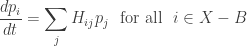

So, the populations 


The off-diagonal entries 

says that the rate for population to transition from one state to another is non-negative. The second:
says that population is conserved, at least if there are no boundary states. Population can flow in or out at boundary states, since the master equation doesn’t hold there.
A steady state is a solution of the open master equation that does not change with time. A steady state for a closed Markov process is typically called an equilibrium. So, an equilibrium obeys the master equation at all states, while for a steady state this may not be true at the boundary states. Again, the reason is that population can flow in or out at the boundary.
We say an equilibrium 

Suppose we’ve got an open Markov process that has a detailed balanced equilibrium 


Definition. Given an open Markov process with detailed balanced equilibrium
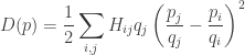
This formula is a bit tricky, but you’ll notice it’s quadratic in 
Using this concept we can formulate a principle of minimum dissipation, and prove that non-equilibrium steady states obey this principle:
Definition. We say a population distribution 


Theorem 1. A population distribution 

Proof. This follows from Theorem 28 in A compositional framework for Markov processes.
Minimum entropy production versus minimum dissipation
How does dissipation compare with entropy production? To answer this, first we must ask: what really is entropy production? And: how does the equilibrium state
The relative entropy of two population distributions 

It is well known that for a closed Markov process with 
• John Baez and Blake Pollard, Relative entropy in biological systems. (Blog article here.)
We say ‘relative entropy’ in the title, but then we explain why ‘relative information’ is a better name, and use that. More importantly, we explain why
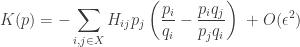
Blake has a nice formula for how fast
Theorem 2. Consider an open Markov process with 


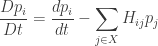
measure how much

Moreover, the first term is less than or equal to zero.
Proof. For a self-contained proof, see Information geometry (part 15), which is coming up soon. It will be a special case of the theorems there. █
Blake compares this result to previous work by Schnakenberg:
• J. Schnakenberg, Network theory of microscopic and macroscopic behavior of master equation systems, Rev. Mod. Phys. 48 (1976), 571–585.
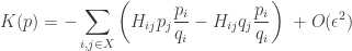
The negative of Blake’s first term is this:

Under certain circumstances, this equals what Schnakenberg calls the entropy production. But a better name for this quantity might be free energy loss, since for a closed Markov process that’s exactly what it is! In this case there are no boundary states, so the theorem above says 
For an open Markov process, things are more complicated. The theorem above shows that free energy can also flow in or out at the boundary, thanks to the second term in the formula.
Anyway, the sensible thing is to compare a principle of ‘minimum free energy loss’ to the principle of minimum dissipation. The principle of minimum dissipation is true. How about the principle of minimum free energy loss? It turns out to be approximately true near equilibrium.
For this, consider the situation in which

for some small numbers 

Theorem 3. Consider an open Markov process with

where 


Proof. First take the free energy loss:

Expanding the logarithm to first order in 
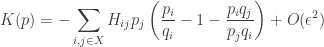
Since 

or
Since 

Next, take the dissipation
and expand the square, getting

Since 


Since 


This matches what we got for 

In short: detailed balanced open Markov processes are governed by the principle of minimum dissipation, not minimum entropy production. Minimum dissipation agrees with minimum entropy production only near equilibrium.


Interesting, thanks for posting. In continuum thermomechanics there are principles often used to obtain constitutive equations – maximum dissipation and/or maximum entropy production. From memory these aren’t always equal, the difference being related to failure of Onsager symmetry and subtleties of othogonality conditions. Zeigler and Edelen are two names that commonly associated with these ideas.
Any relation to this work? Is the min/max a sign thing, different constraints or a micro/macro principle difference?
PS have you looked at the GENERIC approach which has a chapter in the Jou et al book you mention? I’d be curious to hear your take since it’s supposed to be based on Hamiltonian/symplectic/contact structures etc.
I find it surprising to hear that maximum dissipation or maximum entropy production are often used in continuum thermomechanics: in systems near equilibrium people often use minimum entropy production. The idea of maximum entropy production seems to be much more speculative: I’ve seen it championed by Roderick Dewar in biology and climate science.
On the other hand, the usual ‘derivations’ of minimum entropy production involve Onsager reciprocity, so I can easily this principle gets replaced by something subtler when that fails. For us, the thing analogous to Onsager reciprocity is the detailed balance condition, which says a certain matrix is symmetric:
so if we define
then this matrix is symmetric.
I’ve looked into the GENERIC approach just a bit, and I wrote a bit about it in ‘week295’ of This Week’s Finds. Go down to my discussion of
• Hans Christian Öttinger, Beyond Equilibrium Thermodynamics, Wiley, 2005.
This would usually be in the context of a framework involving a free energy function, a dissipation function and an additional closure assumption relating these parts (similar to but not nec the same as GENERIC). Most standard models of eg visco-elastic-plastic materials can be derived in these terms. I took a course quite a few years ago now where we went through all the usual materials models from this perspective.
Ziegler’s book Introduction to Thermomechanics has many examples I think. It’s certainly popular in the field of plasticity. See eg ‘Principles of Hyperplasticity’ by Houlsby and Puzrin for example. Edelen’s book ‘Applied Exterior Calculus’ also has a chapter on thermodynamics and includes a derivation of terms which violate Onsager symmetry.
Thanks for the link to your discussion of Öttinger’s Beyond Equilibrium Thermodynamics btw. I own it but haven’t yet read it in any detail.
Your review mentions that these ideas might be related to Dirac structures. I believe Appendix B of the book has material on these. It’s a bit beyond my current knowledge to comment any further though.
One last ref (sorry to spam) – Ostoja-Starzewski is a generally pretty clear contemporary worker in continuum thermomechanics who is familiar with both Ziegler and Edelen’s work as well as stochastic mechanics problems.
A recent paper of his includes all these elements: ‘Continuum mechanics beyond the second law of thermodynamics’ at http://m.rspa.royalsocietypublishing.org//content/470/2171/20140531
Over on G+, John Wehrle wrote:
The basic idea of ‘dissipation’ is that it’s the rate at which things ‘run down’. For example, if you wind up a clock it ticks and ‘runs down’ until it stops.
A bit more formally, dissipation is something like the rate of decrease of ‘free energy’. Free energy is energy in useful form: energy that can be used to do work. It has a number of precise definitions, but roughly, it’s energy that’s not in the form of heat.
However, when we try to make the idea of dissipation completely precise, we find that there are a number of different quantities, all with some right to the name ‘dissipation’, which are almost equal for systems near equilibrium, but significantly different far from equilibrium. And then the question becomes: which one is right for which purpose?
Can you recommend any other books (aside from Öttinger’s) about nonequilibrium thermodynamics?
Ilya Prigogine has written an approximately infinite number of books on nonequilibrium thermodynamics—like, more than 8. Since he won the Nobel Prize for his work on this subject, and since he was the one who really emphasized how ordered structures can appear in nonequilibrium systems, I think some of his books would be the best way to get a feel for the subject. I haven’t read this particular one, but people seem to like it:
• Dilip Kondepudi and Ilya Prigogine, Modern Thermodynamics: From Heat Engines to Dissipative Structures, Wiley, 1998.
He also has good books of a somewhat more ‘pop’ nature, like this:
• Ilya Prigogine and Isabelle Stengers, Order Out of Chaos, Bantam, 1984.
I read the one by Kondepudi and Prigogine, and it’s pretty good. The explanations are generally very clear and easy to follow. There’s a lot of focus on systems of chemical reactions. There’s almost no mention of statistical mechanics though (I think Prigogine might have developed some skepticism about the usual statistical interpretation of thermodynamics in his later years, which maybe explains this), and a lot of time is spent on equilibrium thermodynamics. It adopts a ‘non-equilibrium friendly’ entropy production formalism from the start though, and covers the linear phenomenological laws, the Onsager reciprocal relations, non-equilibrium steady states, minimum entropy production, and so on, with refs to more info.
Can you say much about how Donsker-Varadhan results and Large Deviations tie into this? It really looks like this covers similar ground, but I don’t see any connections made. Quite possibly I am just missing a lot.
I don’t know anything about ‘the Donsker–Varadhan results’ except what I just read right now, but it seems quite different than what Blake is doing. The Donsker–Varadhan result I just read is a general result about random variables, while Blake’s work amounts to a characterization of steady states of detailed balanced open Markov processes. The only thing I see in common is that they mention relative entropy. But Blake’s work shows that steady states of detailed balanced Markov processes are not characterized in terms of relative entropy, but instead in terms of dissipation! (More on that in Part 16.)
Here’s what I just learned about Donsker–Varadhan.
Theorem. Suppose is a bounded measurable function on a probability measure space
  with measure
  . Then
where is the relative entropy:
and we’re taking the supremum over probability measures Moreover, the probability measure
  that achieves the supremum is the one with
All this looks hugely like the usual concept of a Gibbs state, also known as a Boltzmann distribution in statistical mechanics: this is the probability distribution that minimizes free energy, which is essentially the same as relative entropy, and it’s given by a formula that’s identical to the equation above—though usually the notation is quite different, making this a bit hard to see.
So, I’d say is a Gibbs state, and the Donsker–Varadhan formula is a formula for the logarithm of the partition function… a quantity that physicists know and love.
However, the Donsker–Varadhan result seems to be applied to ‘large deviations’. The point is that the quantity
tells us something about the probability that gets really big.
You wrote:
Does the “we” mean that this is a new definition of dissipation?
Is there some formula which expresses the disspation so that the impact of boundary states is better visible, similar to the one for the relative entropy? In particular I could imagine that for certain boundary conditions dissipation might not have a minimum.
Did you also look at maximum disspation? That is I don’t know wether a matching notion of dissipation is meant here, but some people seem to want to relate maximum dissipation to self-organisation, at least thats what I understand from this pop science article.
Nad wrote:
Yes. At least it might be slightly new — the literature is huge and it’s hard to tell. We introduced this definition in our paper A compositional framework for Markov processes. But there we showed how any detailed balanced Markov process could be mapped to an electrical circuit made of resistors. We showed that then the dissipation of such a Markov process equals the power consumed by the corresponding circuit.
Maybe. I’ll think about that. We’re planning to write another paper about this stuff.
No, it always has a minimum, since it’s a sum of squares times positive numbers.
No, because it can be arbitrarily large.
For similar reasons, the principle of maximum entropy production seems incoherent to me. There’s also no reasonable derivation of this principle.
Is it the same definition as in Prigogine?
yes, now I remember, I briefly glanced at the paper.
?? But could be negative.
It’s seems that due to the detailed balanced condition for an equilibrium dissipation turns into a quadratic form, but I can’t even see that its positive definite, but maybe I oversaw something.
oops yes thats true :)
Nad wrote:
Prigogine has written about 10 books and lots of papers, and I haven’t read all of them. But I’ve never seen our definition of dissipation in anything he wrote or anything anyone else wrote. That’s why I said it “might be slightly new”.
If I were less experienced, I would have said our definition is new. But I’ve learned how hard it is to invent something simple that nobody has ever thought of before.
Did he give at all a definition of dissipation?
experienced? could also be due to culture and/or character.
Anyways I haven’t yet figured out how “complete” the correspondence between electrical circuits and the above Markov processes is. Part of the problem is of course that I do not understand that category theoretic language and that I can’t find the time to learn it. I find in particular confusing that if you have an edge between two points i and j then there could be a flow on the edge
  (as defined in your article) but no flow from j to i, which makes the analogy between current and flow (see analogy table in your article) a bit hard to see. But maybe I haven’t right understood what you mean here that is in particular by my brief browsing I couldn’t find a definition of
  but just what you call “flow law” which -if you call it “law”- seems in particular to be not a “definition”.
Moreover you relate the “flow law” to Ohms law and that analogy I also dont really see.
Nad wrote:
Again, I haven’t read everything he wrote. But in the book I’m reading now, Modern Thermodynamics, he defines quantities called ‘entropy production’ and ‘excess entropy production’ which are somewhat similar to our ‘dissipation’, but also somewhat different. In particular, he’s working in the context of thermodynamics rather than statistical mechanics, so he doesn’t have probabilities or Markov processes.
(For anyone who has this book, look at equation 18.3.6, which is a formula for ‘excess entropy production’: it looks a lot like the quantity
which we discuss in Part 16 of this series. But they have different meanings, since ours is defined in terms of probabilities and his is not.)
We explain this issue, and various other tricky issues in the analogy between circuits and detailed balanced Markov processes, in the conclusions to our paper with Brendan. Very very briefly, current can flow in either direction along an edge in a circuit, while probability can only flow in one direction along an edge in a Markov process, so the detailed balanced Markov process analogous to a specific circuit needs to have two edges for each edge of the circuit.
But please read the conclusions if you want my real thoughts on this analogy! Category theory is the way to make analogies into actual mappings (functors), so our paper is all about a functor from detailed balanced Markov processes to circuits, but in the conclusions we try to avoid talking about functors.
I don’t think I ever said “flow law”. I don’t know what you mean by “flow law”.
Detailed balanced Markov processes do obey a law analogous to Ohm’s law.
In the conclusions: In the analogy table on page 38. there the “flow law” is listed as an analogy to Ohms law.
I saw the text, in the conclusions, but unfortunately it didn’t help to answer the above questions.
Oh, okay. I guess I made up the name “flow law” to make it sound more analogous to “Ohm’s law”. That was silly.
This law is just the master equation in disguise. We should call it the master equation.
I have thought about that but this is all not so clear to me.
Current is usually the time derivative of charge. So is the current in a electric circuit defined to be the time derivative of the different potentials (“the charges”) at the two vertices of an edge?
Then yes Ohms Law would give you a “master equation” for the differences of potentials, i.e. an equation which “lives” on an edge. But the time differential of the differences of population deviations between two vertices along an edge would give for the Markov Master equation a sum over all sorts of edges.
Apart from that it seems the detailed balance condition says something about the connection between vertices and not about the seperate edges….but as said I skipped the category part.
Here is the article by Jeremy England to which the pop science article refers:
Click to access 2013jcpsrep.pdf
The big differerence is that he is considering the early stages of a Markov process, starting with a single cell in a closed (but friendly) system. A somewhat mangled quote (from PDF) follows:
See Fig 1 in this paper: http://www.cs.cornell.edu/cv/researchpdf/19ways+.pdf. Jeremy England is looking at the left end of the graph, well before s/m. John and Blake are looking at the right end.
thanks Graham, I actually just wanted to get an overview and I don’t understand your last comment.
I briefly looked into the cpsrep.pdf but I know already by first sight, that it would take me way too much time to understand it.
There seems also a lot of guess work necessary, like is the S in equation (2) entropy? If yes what kind of entropy? a.s.o.
I searched whether the term dissipation shows up and it didn’t so its not even possible for me to see how on earth this article relates to the pop science article.
It almost sounds from this like we’re studying death and decay, but in fact there are many processes in living systems that can be (approximately) modeled by ‘nonequilibrium steady states’: processes where something flows in one end and out the other end at a constant rate. This is more interesting than ‘equilibrium’ but less interesting than truly dynamic processes, where flows change with time.
There’s a lot of work on nonequilibrium steady states in thermodynamics, and we’re trying to gather it up and package it in our formalism. What’s mostly interesting to us is how you can take a nonequilibrium steady state on a big complicated network and think of it as built from nonequilibrium steady states on the pieces: category theory helps formalize this.
Nonequilibrium steady states are a lot more interesting than equilibrium (the bread and butter of classical thermodynamics) but less interesting than truly dynamical processes: life in all its pulsing, throbbing splendor. We are working our way up the ladder of interestingness, and in a while we’ll start talking about truly dynamical processes, always taking the network viewpoint.
Heh. I didn’t mean to suggest you’re studying death and decay, at least not exclusively. I imagine your nonequilibrium steady states would have equal amounts of birth and death.
Lately we’ve been thinking about open Markov processes. These are random processes where something can hop randomly from one state to another (that’s the ‘Markov process’ part) but also enter or leave the system (that’s the ‘open’ part).
The ultimate goal is to understand the nonequilibrium thermodynamics of open systems—systems where energy and maybe matter flows in and out. If we could understand this well enough, we could understand in detail how life works. That’s a difficult job! But one has to start somewhere, and this is one place to start.
We have a few papers on this subject:
• Blake Pollard, A Second Law for open Markov processes. (Blog article here.)
• John Baez, Brendan Fong and Blake Pollard, A compositional framework for Markov processes. (Blog article here.)
• Blake Pollard, Open Markov processes: A compositional perspective on non-equilibrium steady states in biology. (Blog article here.)