The structure of a diamond crystal is fascinating. But there’s an equally fascinating form of carbon, called the triamond, that’s theoretically possible but never yet seen in nature. Here it is:

In the triamond, each carbon atom is bonded to three others at 120° angles, with one double bond and two single bonds. Its bonds lie in a plane, so we get a plane for each atom.
But here’s the tricky part: for any two neighboring atoms, these planes are different. In fact, if we draw the bond planes for all the atoms in the triamond, they come in four kinds, parallel to the faces of a regular tetrahedron!

If we discount the difference between single and double bonds, the triamond is highly symmetrical. There’s a symmetry carrying any atom and any of its bonds to any other atom and any of its bonds. However, the triamond has an inherent handedness, or chirality. It comes in two mirror-image forms.
A rather surprising thing about the triamond is that the smallest rings of atoms are 10-sided. Each atom lies in 15 of these 10-sided rings.
Some chemists have argued that the triamond should be ‘metastable’ at room temperature and pressure: that is, it should last for a while but eventually turn to graphite. Diamonds are also considered metastable, though I’ve never seen anyone pull an old diamond ring from their jewelry cabinet and discover to their shock that it’s turned to graphite. The big difference is that diamonds are formed naturally under high pressure—while triamonds, it seems, are not.
Nonetheless, the mathematics behind the triamond does find its way into nature. A while back I told you about a minimal surface called the ‘gyroid’, which is found in many places:
• The physics of butterfly wings.
It turns out that the pattern of a gyroid is closely connected to the triamond! So, if you’re looking for a triamond-like pattern in nature, certain butterfly wings are your best bet:
• Matthias Weber, The gyroids: algorithmic geometry III, The Inner Frame, 23 October 2015.
Instead of trying to explain it here, I’ll refer you to the wonderful pictures at Weber’s blog.
Building the triamond
I want to tell you a way to build the triamond. I saw it here:
• Toshikazu Sunada, Crystals that nature might miss creating, Notices of the American Mathematical Society 55 (2008), 208–215.
This is the paper that got people excited about the triamond, though it was discovered much earlier by the crystallographer Fritz Laves back in 1932, and Coxeter named it the Laves graph.
To build the triamond, we can start with this graph:

It’s called 
Let’s not worry yet about what these vectors are. What really matters is this: to move from any atom in the triamond to any of its neighbors, you move along the vector labeling the edge between them… or its negative, if you’re moving against the arrow.
For example, suppose you’re at any red atom. It has 3 nearest neighbors, which are blue, green and yellow. To move to the blue neighbor you add 


Thus, any path along the bonds of the triamond determines a path in the graph
Conversely, if you pick an atom of some color in the triamond, any path in 
Mathematicians summarize these facts by saying the triamond is a ‘covering space’ of the graph
Now let’s see if you can figure out those vectors.
Puzzle 1. Find vectors 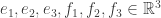
A) All these vectors have the same length.
B) The three vectors coming out of any vertex lie in a plane at 120° angles to each other:
For example, 

C) The four planes we get this way, one for each vertex, are parallel to the faces of a regular tetrahedron.
If you want, you can even add another constraint:
D) All the components of the vectors 
Diamonds and hyperdiamonds
That’s the triamond. Compare the diamond:

Here each atom of carbon is connected to four others. This pattern is found not just in carbon but also other elements in the same column of the periodic table: silicon, germanium, and tin. They all like to hook up with four neighbors.
The pattern of atoms in a diamond is called the diamond cubic. It’s elegant but a bit tricky. Look at it carefully!
To build it, we start by putting an atom at each corner of a cube. Then we put an atom in the middle of each face of the cube. If we stopped there, we would have a face-centered cubic. But there are also four more carbons inside the cube—one at the center of each tetrahedron we’ve created.
If you look really carefully, you can see that the full pattern consists of two interpenetrating face-centered cubic lattices, one offset relative to the other along the cube’s main diagonal.
The face-centered cubic is the 3-dimensional version of a pattern that exists in any dimension: the Dn lattice. To build this, take an n-dimensional checkerboard and alternately color the hypercubes red and black. Then, put a point in the center of each black hypercube!
You can also get the Dn lattice by taking all n-tuples of integers that sum to an even integer. Requiring that they sum to something even is a way to pick out the black hypercubes.
The diamond is also an example of a pattern that exists in any dimension! I’ll call this the hyperdiamond, but mathematicians call it Dn+, because it’s the union of two copies of the Dn lattice. To build it, first take all n-tuples of integers that sum to an even integer. Then take all those points shifted by the vector (1/2, …, 1/2).
In any dimension, the volume of the unit cell of the hyperdiamond is 1, so mathematicians say it’s unimodular. But only in even dimensions is the sum or difference of any two points in the hyperdiamond again a point in the hyperdiamond. Mathematicians call a discrete set of points with this property a lattice.
If even dimensions are better than odd ones, how about dimensions that are multiples of 4? Then the hyperdiamond is better still: it’s an integral lattice, meaning that the dot product of any two vectors in the lattice is again an integer.
And in dimensions that are multiples of 8, the hyperdiamond is even better. It’s even, meaning that the dot product of any vector with itself is even.
In fact, even unimodular lattices are only possible in Euclidean space when the dimension is a multiple of 8. In 8 dimensions, the only even unimodular lattice is the 8-dimensional hyperdiamond, which is usually called the E8 lattice. The E8 lattice is one of my favorite entities, and I’ve written a lot about it in this series:
To me, the glittering beauty of diamonds is just a tiny hint of the overwhelming beauty of E8.
But let’s go back down to 3 dimensions. I’d like to describe the diamond rather explicitly, so we can see how a slight change produces the triamond.
It will be less stressful if we double the size of our diamond. So, let’s start with a face-centered cubic consisting of points whose coordinates are even integers summing to a multiple of 4. That consists of these points:
(0,0,0) (2,2,0) (2,0,2) (0,2,2)
and all points obtained from these by adding multiples of 4 to any of the coordinates. To get the diamond, we take all these together with another face-centered cubic that’s been shifted by (1,1,1). That consists of these points:
(1,1,1) (3,3,1) (3,1,3) (1,3,3)
and all points obtained by adding multiples of 4 to any of the coordinates.
The triamond is similar! Now we start with these points
(0,0,0) (1,2,3) (2,3,1) (3,1,2)
and all the points obtain from these by adding multiples of 4 to any of the coordinates. To get the triamond, we take all these together with another copy of these points that’s been shifted by (2,2,2). That other copy consists of these points:
(2,2,2) (3,0,1) (0,1,3) (1,3,0)
and all points obtained by adding multiples of 4 to any of the coordinates.
Unlike the diamond, the triamond has an inherent handedness, or chirality. You’ll note how we used the point (1,2,3) and took cyclic permutations of its coordinates to get more points. If we’d started with (3,2,1) we would have gotten the other, mirror-image version of the triamond.
Covering spaces
I mentioned that the triamond is a ‘covering space’ of the graph 


This automatically means that every path in
If you’re a high-powered mathematician you might wonder if
What does this mean? Any path in 
For example, there’s a loop in

We can turn this into an expression

However, we can’t simplify this to zero using just the commutative law and cancelling like terms. So, if we start at some red atom in the triamond and take the unique path that goes “red, blue, green, red”, we do not get back where we started!
Note that in this simplification process, we’re not allowed to use what the vectors “really are”. It’s a purely formal manipulation.
Puzzle 2. Describe a loop of length 10 in the triamond using this method. Check that you can simplify the corresponding expression to zero using the rules I described.
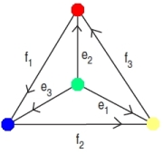
A similar story works for the diamond, but starting with a different graph:
The graph formed by a diamond’s atoms and the edges between them is the universal abelian cover of this little graph! This graph has 2 vertices because there are 2 kinds of atom in the diamond. It has 4 edges because each atom has 4 nearest neighbors.
Puzzle 3. What vectors should we use to label the edges of this graph, so that the vectors coming out of any vertex describe how to move from that kind of atom in the diamond to its 4 nearest neighbors?
There’s also a similar story for graphene, which is hexagonal array of carbon atoms in a plane:

Puzzle 4. What graph with edges labelled by vectors in 
I don’t know much about how this universal abelian cover trick generalizes to higher dimensions, though it’s easy to handle the case of a cubical lattice in any dimension.
Puzzle 5. I described higher-dimensional analogues of diamonds: are there higher-dimensional triamonds?
References
The Wikipedia article is good:
• Wikipedia, Laves graph.
They say this graph has many names: the K4 crystal, the (10,3)-a network, the srs net, the diamond twin, and of course the triamond. The name triamond is not very logical: while each carbon has 3 neighbors in the triamond, each carbon has not 2 but 4 neighbors in the diamond. So, perhaps the diamond should be called the ‘quadriamond’. In fact, the word ‘diamond’ has nothing to do with the prefix ‘di-‘ meaning ‘two’. It’s more closely related to the word ‘adamant’. Still, I like the word ‘triamond’.
This paper describes various attempts to find the Laves graph in chemistry:
• Stephen T. Hyde, Michael O’Keeffe, and Davide M. Proserpio, A short history of an elusive yet ubiquitous structure in chemistry, materials, and mathematics, Angew. Chem. Int. Ed. 47 (2008), 7996–8000.
This paper does some calculations arguing that the triamond is a metastable form of carbon:
• Masahiro Itoh et al, New metallic carbon crystal, Phys. Rev. Lett. 102 (2009), 055703.
Abstract. Recently, mathematical analysis clarified that sp2 hybridized carbon should have a three-dimensional crystal structure (
The picture of the


John, perhaps you will be interested I asked for a more general topic, …Or not here ;) http://chemistry.stackexchange.com/questions/19475/hydrocarbons-with-only-4-carbon-atoms
BTW, I asked that problem to some advanced students at High School…I do know where the triamond is in all the structures, but there are other mysterious stuff…
Puzzle 1
The outgoing vectors at the green vertex are:
These are of equal length, and sum to zero, which means they must be coplanar and all separated by 120°. They are all orthogonal to:
The outgoing vectors at the yellow vertex are:
These meet the same conditions, and are orthogonal to:
The outgoing vectors at the red vertex are:
These meet the same conditions, and are orthogonal to:
The outgoing vectors at the blue vertex are:
These meet the same conditions, and are orthogonal to:
Finally, the four normals to the planes associated with the four vertices:
all have equal lengths and mutual dot products of , so they are the normals to the faces of a regular tetrahedron.
Right! I thought you might like this one.
The descriptions I’ve read don’t emphasize the tetrahedron, but that seems like the right way to understand the triamond. Here’s how I think about it now.
We can take a cube with vertices and inscribe two regular tetrahedra in it.
Pick the one that contains the point as you’ve done. Now we want to find 3 vectors in this plane that are at 120° to each other. It helps to know that the points
  with integer coordinates summing to zero form a triangular lattice, lying in a plane orthogonal to
  So use the vectors
which are at 120° angles since they have length squared 2 and dot product -1 with each other. I could have also used the negatives of these 3 vectors, but I’m deliberately making the same choice as you.
Now, we can use the rotational symmetries of the tetrahedron to carry this triple of vectors to triples that are orthogonal to the other vertices of the tetrahedron.
However, I’m not sure that’s the right method. There’s a sign issue to consider. After all, we could have used the negatives of the 3 vectors above! More importantly, we need the vector pointing from the red vertex of the tetrahedron to the blue one (for example) to be minus the vector pointing from the blue vertex to the red one.
So, I will have to rotate the tetrahedron so that red vertex gets carried to another vertex, say the blue one
  and see what this does to the 3 vectors listed above.
One last thing: you made a couple of choices to get your solution (which tetrahedron inscribed in the cube, which triple of vectors to start with at one vertex). In the end, there should be just two solutions, which give mirror-image versions of the triamond!
Luckily this is easy: this rotation just negates the first two coordinates. So it carries the outgoing vectors at the red vertex, namely
to the vectors
And these are indeed your outgoing vectors at the blue vertex!
So, after choosing a triple of outgoing vectors for one vertex of the tetrahedron, we just rotate them to get the triples for the other vertices. But the interesting thing is that our initial choice has a handedness.
Re: Universal Abelian Covering Space… the image of should be the commutator subgroup;
  is its Deck Transformations (which is transitive on “fibers” because the Commutator Subgroup is Normal)…
So, you’ve told us that there’s a 4-colouring of T, but in connection with the suppressed double-bonds, I’m wondering is T in fact bipartite, like graphene?
Also, is there a predicted X-ray crystalogram for this gem?
Oh, I can answer bipartite: yes, because commutators are made of an even number of oriented edges possibly canceling in pairs, so loops in T must be even.
Jesse wrote, with more Capital Letters:
Good, right! I had said some silly stuff, mixing up subgroups and quotient groups as I often do when dealing with covering spaces and Galois theory. I realized my mistake while eating breakfast, then ran back and deleted it. But now I will add a correct explanation, and a new puzzle.
That’s an interesting question.
The graphene graph is bipartite because it’s a covering space, in fact the universal abelian cover, of a graph that’s bipartite. Finding that graph is Puzzle 4.
Similarly, the diamond graph is bipartite because it’s a covering space, in fact the universal abelian cover, of this bipartite graph:
The triamond graph doesn’t have this reason for being bipartite. It’s the universal abelian cover of
  which is not bipartite:
The triamond graph inherits a 4-coloring from the 4 colors of vertices shown here, and it inherits single and double bonds from the two kinds of edges shown here. However, each vertex of any color is connected by edges to vertices of all the other 3 colors.
This doesn’t prove the triamond graph is not bipartite! Indeed, while has lots of cycles of odd length — forbidden in a bipartite graph — the shortest cycles in the triamond graph has length 10.
So, my answer to your question is “I don’t know.”
(Meanwhile, you have answered it: “yes”.)
I don’t know that either!
Think diamond is fascinating, how about the zincblende crystal structure? That one is partly responsible for the high-speed optoelectronics advances made over the last few decades.
Zincblende is precisely a diamond structure but for one substitution rule. It also forms spontaneously with no pressure required.
I’m not sure what “one substitution rule” means. I just checked, and the zincblende crystal structure looks just like diamond, except we have alternating zinc and sulfur atoms:
Maybe that’s what “one substitution rule” means.
I mentioned that in diamond we have “two kinds of atoms” — more precisely, atoms lying in two separate face-centered cubic lattices. Diamond has a symmetry carrying one of these lattices to another. But in zincblende one lattice is zinc atoms and the other is sulfur!
Zinc sulfide also comes in another form, called wurtzite, which has hexagonal rather than cubic symmetry:
Is there are “universal abelian covering” description of this one?
Column III + Column V elements for zincblende and Column IV for diamond.
Watch what happens when you have a free surface on [100], [111], or [110] orientations.
There is a possibility of creating a direct-bandgap lattice out of a column IV diamond structure. Add tin to germanium and one can potentially create an infared laser. Years ago, I was the first to successfully create a metastable SnGe lattice, which we confirmed via x-ray crystallography,
Applied Physics Letters 54(21):2142 – 2144 · May 1989
Since that time others have made progress in improving the opto-electronic properties of this material.
Who knows what kind of interesting electronic properties would arise with these hypothetical lattice structures.
A.F. Wells in addition to his modest The Third Dimension in Chemistry (1956) wrote a massive textbook on Structural Inorganic Chemistry (1962, OUP) that may be worth dipping into. Some content may be available on Google Books, but you can never tell how much! (GB always truncates you on the interesting page). With luck, you may find discussion Diamond-type structures around p120.
I was confused until it sunk in that you said each vertex in K4 represents a kind of atom, not an atom of a specific kind, so that e.g. edge f2 notwithstanding, the blue and yellow triamond atoms bonded to a given red are not bonded to each other. (You also said the smallest ring was 10 atoms, so I have no good excuse:-).
I spent a good 10 minutes debating whether to add this sentence:
I couldn’t tell whether it would enlighten people or confuse them. You’ve convinced me to add it!
An interesting post: I would not be surprised to find some way of K4 production if some exotic demand arose (say akin to N-induced vacancies in diamond). Indeed, how one would recognise K4 admixed with other carbon allotropes might be the initial challenge. An X-ray diffraction fingerprint perhaps, but that’s so obvious it must be well-studied.
On a minor wikipedian point, the attribution of the K4 image as being “drawn by ‘Workbit'” may be misleading as Sunada on p6 in this book attributes the same image to Kayo Sunada. Copyright on images is a minefield. Sunada also has a 2012 “Lecture on topological crystallography” which has some interesting background for non-mathematicians like myself. Search on Google Scholar for an accessible pre-print.
Thanks! So it’s possible that Workbit just stole this image and put it on Wikicommons here, calling it “own work”.
I’ll guess that Kayo Sunada is a relative of Toshikazu Sunada, who studied and popularized the crystal.
Re Puzzle 5 (unfinished)
In trying to build a small bit of T, starting from the covering space description, I found I needed to use the fact that every edge of a tetrahedron is disjoint from a unique other edge; that particular fact doesn’t work in any other dimension.
On the other hand, K5 certainly has a universal abelian cover, whose deck transformations should be free abelian of rank … (5*4/2)- 5 + 1 = 6. (hmm… that’s also the dimension of O(4)…)
At the end of his fascinating paper, Sunada writes:
This is the one you’re talking about for
The ‘strong isotropic property’ is defined earlier in his paper. If you’ve got a graph embedded in he says it’s strongly isotropic if the group of Euclidean symmetries preserving the graph acts transitively on flags, where a flag is a vertex and an edge incident to that vertex.
An abstract graph having symmetries that act transitively on flags is called a symmetric graph, and there’s a whole literature on these (though maybe this focuses on finite graphs).
So, any strongly isotropic graph embedded in has to be symmetric.
I have an idea for Puzzle 5. Let’s look at the universal abelian covers of some nice graphs, namely those coming from Platonic solids. We got the triamond from the tetrahedron, but this could be an example of a systematic procedure that works for other examples!
The vertices and edges of a cube form a graph which looks like this if you flatten it out:
This graph has 5 independent loops. In other words, its fundamental group is the free group on 5 generators. Its universal abelian cover should thus live in 5 dimensions.
How do we define this? Imagine 6 kinds of atoms, one for each vertex of the cube. Then, figure out vectors that describe how to hop from one kind of atom to a neighboring atom of a different kind. Each atom will have 3 neighbors.
How do we figure out these vectors?
Label the directed edges of the cube with vectors. In other words, draw arrows on the edges, and label them with vectors—but decree that the vector changes sign if we change our minds about which way the arrow points.
Demand that the vectors labeling the 3 edge pointing out of each vertex of the cube sum to zero. This is like Kirchhoff’s current law: it says the total current flowing into each vertex equals the total current flowing out. However, now current is a vector, not a scalar.
How much choice do we have in picking vectors like this?
The cube has 12 edges and 8 vertices. So, we have to choose 12 vectors, but impose 8 equations among them.
That sounds like ultimately we’re picking 12 – 8 = 4 vectors. But that’s wrong, because not all the equations are independent! You can derive the last equation from the rest! So, we’re really picking 5 vectors.
Here’s one way to see this: think of our graph as an electrical circuit, but where current is vector-valued. If we impose Kirchhoff’s current law at every vertex except one, it must also hold at the last one.
Another way to see it is to remember that our graph has 5 independent loops. Each one gives an independent quantity, which electrical engineers would call a mesh current.
Another way to see it is this: since the fundamental group of our graph is the free group on 5 generators, its 1st homology group, the abelianization of the fundamental group is (In fact this is the same idea as the electrical engineering argument, just phrased in another language.)
Anyway, the upshot is this. The task of choosing vectors for edges which sum to zero at each vertex amounts to choosing 5 vectors.
We can make them linearly independent if we use a 5-dimensional vector space. So, we are getting ready to build a graph, say C, embedded in 5d space. This graph will be the universal abelian cover of the graph shown above.
We’d like to choose the vectors in a very nice symmetrical way. At the very least, the symmetries of the cube should act as symmetries of our graph C—and not just symmetries of it as an abstract graph, but as a graph embedded in 5-dimensional Euclidean space.
Hmm, I thought I knew how to do this, but now I don’t.
So that’s a nice challenge. If we succeed we’ll get a very nice crystal in 5 dimensions where each atom has 3 neighbors.
We can also try this for the other Platonic solids:
The tetrahedron gives the triamond graph T, which lives in 3 dimensions, because the tetrahedron has 4 faces—or if you prefer, it has 6 edges and 4 vertices, and 6 – 4 + 1 = 3. In the corresponding crystal, each atom has 3 neighbors.
The cube gives a graph C which lives in 5 dimensions, because the cube has 6 faces—or if you prefer, it has 12 edges and 8 vertices, and 12 – 8 + 1 = 5. The challenge is to find the most symmetrical version of this graph C. In the corresponding crystal, each atom has 3 neighbors.
The octahedron gives a graph O which lives in 7 dimensions, because the octahedron has 8 faces—or if you prefer, it has 12 edges and 6 vertices, and 12 – 6 + 1 = 7. The challenge is to find the most symmetrical version of this graph O. In the corresponding crystal, each atom has 4 neighbors.
The dodecahedron gives a graph D which lives in 11 dimensions, because the dodecahedron has 12 faces—or if you prefer, it has 30 edges and 20 vertices, and 30 – 20 + 1 = 11. The challenge is to find the most symmetrical version of this graph D. In the corresponding crystal, each atom has 3 neighbors.
The icosahedron gives a graph I which lives in 19 dimensions, because the icosahedron has 19 faces—or if you prefer, it has 30 edges and 12 vertices, and 30 – 12 + 1 = 9. The challenge is to find the most symmetrical version of this graph I. In the corresponding crystal, each atom has 5 neighbors.
Of course we can also play this game starting with other polyhedra or polytopes.
For example, the universal abelian cover of buckminsterfullerene should give a purely theoretical crystal form of carbon in 31 dimensions, where each atom has 3 neighbors: two connected with single bonds, and one connected with a double bond.
I wrote:
Okay, I think I get it now. This should work, not just for the cube, but for all the examples. But let me describe it for the cube.
We start by arbitrarily directing each edge in the cube—that is, drawing arrows on them. Then the space consists of ways to label directed edges by numbers. The symmetries of the cube act as linear transformations of this space. The recipe is pretty obvious, I hope—except for one thing. We just need to remember that if we map an edge to an edge in a way that reverses its direction, we stick a minus sign in front of the number labeling that edge! In other words, we’re thinking of
  as the space of ‘electrical currents on edges of the cube’.
If we give its usual inner product, the symmetries of the cube act in a way that preserves this inner product.
Then, let be the subspace consisting of currents that obey Kirchhoff’s current law. As we’ve seen, this is 5-dimensional. We can use our inner product to define a projection
Next, for each directed edge let
let  be the corresponding basis vector, using the standard basis of
Then, let
So, for each directed edge of the cube we get a vector in our 5-dimensional space
  and these vectors obey Kirchhoff’s current law. That is, when we take the 3 edges directed outward from any vertex in the cube, the corresponding vectors
  sum to zero.
The inner product on gives an inner product on
  and since I haven’t broken the symmetry at any stage of this construction, all the vectors
  will have the same length.
Now, following my previously described recipe, we can build a crystal in 5 dimensions which has 6 kinds of atoms—one for each vertex of the cube. Each atom will have 3 neighbors joined to it by bonds. These bonds will all be the same length, and they will lie at 120° angles from each other.
Since I haven’t spoiled the symmetry at any stage of this construction, the symmetry group of the cube will act on this crystal. Moreover, this crystal—which is really a graph embedded in 5d Euclidean space—will be the universal abelian cover of the graph coming from a cube.
I see two things that could go wrong with this construction.
First, we might have for some
  and thus for all
  due to the symmetry. This would be a major bummer, but I don’t think it happens.
Second, the graph C that we build in 5 dimensions might have vertices that are dense in 5-dimensional space. This would make it not like a ‘crystal’, but it could still be somewhat interesting. I don’t see how to rule out this scenario without some computations. In fact, this scenario reminds me of how we can build quasiperiodic tilings by projecting a hypercubic lattice from n dimensions down to 2 dimensions and then doing some other stuff:
• Greg Egan, de Bruijn.
What if you picked a simplex centred at the origin in and arbitrarily associated each vertex with a face of the cube? Using these six vectors as the vector-valued mesh currents associated with the (oriented) faces of the cube, you then get a vector in
  for each directed edge, as the difference between the vectors associated with the two faces incident on that edge.
I think that might give the same result as your construction, but it would circumvent the need to work in . The symmetries of the cube would act in
  by permuting the vertices of the simplex.
Does that sound right, or have I misunderstood something? In any case, I can try to figure out what kind of graph this produces in .
.
Interesting idea! Maybe that will give the same result, or maybe it will give a different, more symmetrical graph in that has all permutations of a 6-element set as symmetries, rather than merely the symmetries of the cube. The only bad thing I can imagine about getting a more symmetrical graph is that maybe its vertices will be dense in
  , which isn’t what I’d like for the atoms in a crystal—or, less romantically speaking, a sphere packing, possibly a rather loose sphere packing.
Speaking of sphere packings, I just saw George Hart’s picture of the ‘Heesch–Laves loose-packing’ of sphere:
on a page about structures related to the triamond:
• George W. Hart, The (10,3)-a network.
The (10,3)-a network is another name for the triamond graph. I don’t know where this name comes from.
The Heesch–Laves loose-packing was at one point, at least for a time, the least dense packing known of equal-sized spheres in such that each sphere is unable to move if we hold its neighbors fixed. It has a density of about 0.05. For more information see:
• Joseph O’Rourke, Are there locally jammed arrangements of spheres of zero density?, MathOverflow.
1) Naively eyeballing this, I don’t see any spheres which look immobile if their neighbors are fixed. I suppose hidden or omitted (beyond-cell-boundary) spheres could account for all of this, but it seems unlikely (it takes 4 contact points,not all in the same hemisphere to fix a sphere, right?)
2) This kind of thing seems like it could make a compelling museum exhibit (perhaps not a hands-on one, though:-)
Oh, I was being a bit silly: I thought nothing in your construction would break the symmetry down from the permutation group on 6 letters to the symmetry group of the cube, because you’re picking your 6 mesh currents in a way that doesn’t mention the cube. But when you define currents for the cube’s edges, you’re using the way the 6 faces of the cube are incident to its 12 edges. So this could easily break the symmetry down to that of a cube. So it’s possible your construction gives the same result as mine, though I don’t feel sure.
If I find the vector-valued edge currents by projecting the standard basis of into the 5-dimensional subspace of vectors that obey Kirchhoff’s law at all the vertices, and then solve for the vector-valued mesh currents in the same 5-dimensional subspace, then, although the edge currents all have the same lengths, and the mesh currents all have the same lengths … the mesh currents don’t lie at the vertices of a 5-simplex.
But there might be another choice of basis of that yields a 5-simplex.
Using the method starting with the mesh currents at the vertices of a 5-simplex, I did a million-step random walk on the cube’s edge graph and lifted it into . The resulting points look like a discrete set, with none of them closer to each other than the graph’s edge length.
Excellent! Since they’re not bunching up in a nasty way, I suspect the vertices of this graph, call it C, lie in some lattice L in That’s how it works with the triamond: we can start with the lattice of points with integer coordinates, and take ‘half’ of these points in a periodic way.
So, I’d like to figure out the lattice L. Since you built everything starting with the 5-simplex, and the symmetry group of the 5-simplex is the Coxeter group , the obvious guess is the
  lattice.
I think the coordinates of the vertices of a 5-simplex in involve some irrational numbers, since the angle between any two vertices is
  Irrational numbers make me a bit queasy when I’m trying to show something has a periodic pattern.
Luckily, we can work abstractly and simply let L be the lattice consisting of integer linear combinations of the vertices of the 5-simplex. The last vertex is minus the sum of the rest, so this is really a lattice.
These vectors are your ‘mesh currents’. Your edge currents are certain sums of pairs of these. So yes, the vertices of your graph C will clearly form a subset of the lattice L.
(Is it really that easy? When I started writing this I thought it would be harder.)
The next question is: which subset? Or at least: what fraction of the points of L are in this subset, and what is the periodicity of this subset?
The triamond vertices are a subset of the lattice of points with integer coordinates, containing 1/8 of the points. This subset has periodicity 4 in each coordinate direction, but we can also add to a triamond vertex and get another triamond vertex. In other words, we can add
  to any triamond vertex and get another triamond vertex.
If we take any loop in the cube’s edge graph that visits all 8 vertices, and sum the associated edge vectors around the whole loop, we should get a vector in that, when added to any vertex of the covering graph, will take us to another vertex of the covering graph. In fact, adding such a vector should always take us to another vertex of the same colour (in the sense that it covers the same vertex of the cube).
I think the set of all such vectors should form a lattice. If you go around any loop an integral number of times (going backwards for negative integers), that corresponds to multiplying the associated vector by that integer. And you can “add” any two of these all-vertex loops by switching between them at any vertex, which will correspond to adding the associated vectors.
It’s a bit tricky finding a basis for this lattice. By looping around the two faces in each of the 3 pairs of opposite faces of the cube, either in the same direction or in opposite directions, and then stitching those two loops together by going back and forth along any edge that joins them (which cancels out that edge’s vector, since you traverse it both ways), you can systematically get 6 loops that visit every vertex, and any 5 will give linearly independent vectors.
But you can get another set of 5 vectors by a different approach. If you take two identically-positioned “U”-shaped paths on opposite faces of the cube, you can then join the free ends of the “U”s, making an eight-edged loop that visits all 8 vertices without backtracking. There are 12 ways to do this (3 choices of the pair of faces that have the “U”s, then 4 choices for the way you orient the “U”s), but of course there can only be 5 linearly independent vectors arising from them.
Now, neither set of 5 vectors lies wholly in the lattice spanned by the other set of 5. So unless I’m confused, the lattice we need will be the union of both lattices. A basis for the union can be found by taking the union of the bases and reducing it to Hermite Normal Form, which is the analog of reduced row echelon form over the integers.
If I’m right about all of this, I end up with a basis with a determinant that is 2304 times that of the basis for L, the lattice of integer-linear combinations of the 5-simplex vertices. But we have 8 disjoint lattices like this, one for each of the 8 vertex colours. So I’m guessing that 1 in 2304/8 = 288 points of L are vertices of the covering graph.
Ah, I just realised that there’s a much simpler way to get the basis for the loops that visit all 8 vertices. You can just loop around any single face of the cube, but then add self-cancelling detours from each of the four vertices of that face to the closest vertex on the opposite face.
It almost seems like cheating, but these really are loops that visit all 8 vertices, despite the fact that the final vector is a sum of just four edge vectors. And if you pick any 5 faces of the cube, the 5 vectors you get really do give you a basis for the lattice I mentioned previously.
This also makes for a more persuasive case that the previous analysis didn’t miss any points when trying to calculate the density of the covering graph vertices in the lattice L. I argued that any vector that arises from an 8-vertex loop will take you between two identically-coloured vertices of the covering graph … but what about loops that visit less than 8 vertices? They should also give vectors that take you between vertices of the covering graph, so long as you’re starting from a vertex whose colour is one that was included in the loop.
But since looping around a single face of the cube, visiting just 4 vertices, yields the same vector as a loop that visits all 8 vertices, the vectors from those smaller loops are automatically part of the same lattice, and there are no extra points to be counted.
As a cross-check for the methods I’ve used with the cube, I applied the same approach to the tetrahedron, and it did yield the known results for the triamond.
There’s one potentially confusing wrinkle: with the choice of scale we’ve been using for the triamond, the 3-simplex of mesh currents gives a lattice L whose fundamental domains have a volume half that of the lattice with integer coordinates. The lattice of vectors that take you between identically coloured vertices of the covering graph has a density of 1 in 64 points of L, and given the four colours for the four vertices of the tetrahedron, that means 1 in 16 points of L are vertices of the covering graph. But since L is twice as dense as the lattice with integer coordinates, we end up with the required density for the covering graph of 1 in 8 points with integer coordinates.
Greg wrote:
I was confused by this, because I didn’t think it was necessary for the path to visit all 8 vertices. I thought any loop would be okay.
But now maybe I see what you mean. Let’s call the covering graph in the crystal. Let’s call a vertex of this graph an atom, and save vertex to mean ‘vertex of the cube’. There’s a map from atoms to vertices. For each vertex
  of the cube, I’ll call the atoms that map to it atoms of color
For each vertex in the cube and any loop starting at the vertex, we get a vector in
  that when added to any atom of color
  takes us to another atom of color
But you were looking for vectors that when added to any atom give another atom of the same color. For this you chose loops that visit all 8 vertices. You never quite explained why, but I think I see why: these loops can be viewed as starting at any vertex of the cube, and we get the same vector regardless.
At first you thought this condition of visiting all 8 vertices was a serious restriction. But then you decided it was not:
The upshot is that any loop in the cube gives a vector which when added to any atom takes us to another atom of the same color.
So, while the atoms in our crystal do not form a lattice, we can determine a lattice that acts on our crystal as translation symmetries. This lattice consists of integer linear combinations of vectors coming from loops in the cube.
And as you note, there’s nothing special about the cube here! The arguments are very general and should apply to all the cases I mentioned, and others too. I’m glad you checked the tetrahedron.
John wrote:
Right, and it took me a while to grasp that! It seems counter-intuitive at first that the vector from a red-green-blue-red loop can be added to a yellow atom to take you to another yellow atom. It’s only once I realised that a loop of any size gives the same vector as some other loop that visits every vertex (and hence can be thought of as a path that starts and ends at any vertex) that the lattice of translation symmetries made sense.
I am thinking that the structure of the triamond is similar to the structure of the benzene, there is a double bound and two single bound, so that there may be a structure with a resonance.
I am thinking that the triamond could be a phase of right temperature and pressure of carbon, so the spectrum could be observed in carbon star with some masses.
That would be great! As you may know, there was a controversy over whether a certain carbon-rich ‘super-Earth’ planet was made of diamond:
• Megan Gannon, Diamond super-planet may not be so glam, Space.com, 13 October 2013.
There are also discussions of liquid carbon oceans with diamond
icebergs on Neptune and Uranus:
• Eric Bland, Diamond oceans possible on Uranus, Neptune, Discovery.com News, 15 January 2010.
So besides carbon-rich black dwarf stars there are a variety of places where triamonds may lurk—if they are ever stable under any conditions.
Let me try to summarize and generalize some of Greg’s and my discoveries.
Consider a graph drawn on a compact connected oriented surface. So, we have a set
  of vertices, a set
  of edges and a set
  of faces, which are polygons. The faces are oriented in a consistent way, and let’s arbitrarily choose an orientation for each edge.
A good example would be a Platonic solid, or this graph with 24 vertices, 84 edges and 56 triangles that Greg drew on Klein’s quartic curve:
The graph has a universal abelian cover:
and it seems we have a nice way of building this cover and embedding it in where
where  is the number of faces.
To do this, we choose vectors in
in  one for each face
  We demand that they are linearly independent except for one relation: they sum to zero. The nicest way is to choose these vectors to be vertices of a regular simplex in
Then we define a vector for each edge
  to be the difference of vectors for the two faces that
  touches. The orientation we’ve chosen for the edge
  will be consistent with the orientation of one of these faces, say
  and it will go against the orientation of the other face, say
  So, we define
We write for the edge
  equipped with the opposite orientation, and set
Now, we define as follows. We arbitrarily choose a vertex
  For any path of edges
  starting at
  and ending at some vertex
  we get a vector
Here each edge can be either
  or
or  for some
  In other words, we can build paths using edges that either follow the direction we originally chose, or go backwards.
Each vector we get this way will be a vertex in and our covering map
will send it to the vertex the endpoint of the path.
We decree that two vertices are connected by an edge iff there is an edge in
  between
  and
and 
Note that if the edge goes from the vertex
  to the vertex
  , then
Let be the set of vertices of the covering graph
  and let
  be the set of edges of
The set is not usually a lattice: for example, we can get the pattern of atoms in graphene, a diamond or a triamond by this recipe.
However, there’s a lattice generated by all the vectors
  labelling faces. And Greg’s argument shows that
  acts by translations on
[EDIT: No, we should let be the lattice generated by the vectors
where are the edges forming a loop going around the face
  in the direction that matches the orientation of that face.]
In interesting cases we will have a finite group acting as symmetries of our oriented surface, preserving the graph
  For example, this could be the symmetry group of a Platonic solid, or the 168-element group of symmetries of the graph on Klein’s quartic curve.
In this case, we can define for each group element a linear transformation of that permutes the face vectors
  This gives a representation of
  on
on  which preserves the covering graph
  , and also the lattice
Suppose the group acts in a flag-transitive way on the graph
  — that is, mapping any flag (vertex-edge pair, with the vertex incident to the edge) to any other flag. This happens in the highly symmetrical situations I keep using as examples.
Then I believe the semidirect product acts in a flag-transitive way on
The most interesting case is when acts as orthogonal transformations of
  Then
Then  will act as Euclidean transformations: that is, transformations that preserve angles and distances. I believe we can achieve this by choosing the face vectors
  to be vertices of a regular simplex. Then any permutation of the faces will define an orthogonal transformation of
So, we get a bunch of examples of extremely symmetrical higher-dimensional crystals, which are not lattices! Sunada calls a graph in strongly isotropic if there are Euclidean transformations acting on it in a flag-transitive way. We’re getting a lot of examples of these.
Thanks for writing this great summary! But I don’t think you meant to say this part:
The lattice defined this way contains translations that won’t preserve
  . The lattice of translations that act on
  is a sublattice of
  generated by the vectors associated with loops in
  . Even though we can think of each face as defining a loop, the sum of the edge vectors around each face is not the same thing as
  , the “mesh current” associated with that face!
Hmm, I thought it was, but I don’t see any reason it should be.
This confusion of mine feels connected to my confusion here:
A few more points:
1) I didn’t prove all the claims here, e.g. the claim that is the universal abelian cover of
2) I’m not seeing where exactly we use the fact that the vectors sum to zero! This is annoying.
3) I think there should be a fairly simple formula for the density of the vertices inside the lattice
  : that is, the fraction of lattice points that are vertices of the covering graph
  It should depend only on the original graph
  and the surface it’s drawn on.
On (2), if the “mesh currents” don’t sum to zero, you don’t get a consistent system of linear equations for the edge vectors.
On (3), the simplest formula I can give right now for the fraction of points in the lattice
  that belong to the set of vertices of the covering graph is:
where is the number of vertices of the graph
  , and
, and  is the matrix of coordinates for a set of
  loop vectors associated with all but one face of the graph, expressed in a basis
  of “mesh currents” for the same faces.
I don’t know if there’s a simpler way to describe that determinant. Of course it doesn’t depend on the particular vectors we choose for the roles of in
in  , and I believe it’s an invariant of
  alone, at least up to a sign. But I don’t know a slicker way to compute it than solving for the edge vectors and summing them to get the loop vectors.
Greg wrote:
That’s what I felt, but the formula saying the edge current is a difference of mesh currents seems perfectly well-defined regardless of what those mesh currents are. I think something else bad happens if the mesh currents don’t sum to zero.
John wrote:
You’re right, sorry. The bad thing that happens is that the edge currents won’t obey Kirchhoff’s law at every vertex unless the mesh currents sum to zero. There are only free parameters in the solution space for Kirchhoff’s law, so if you want to solve for edge currents obeying that law by using mesh currents, you’re only free to choose
  of them.
Greg wrote:
Right. This mattered to me a lot when I started developing these ideas using the analogy to circuits, but I’m not sure what it does for us when it comes to building a symmetrical crystal.
Of course, one thing it does is ensure that the vectors from any atom to its officially designated neighbors sum to zero. This is a nice property, but not something I’d require in a crystal. More important is that the lengths of these edges are all equal: this is required if we want an edge-transitive symmetry group.
(By the ‘officially designated neighbors’ of an atom, or vertex in I mean those connected to it by edges in
  These are not necessarily the nearest vertices.)
Another thing it may do is this. We have two collections of vectors, which I managed to mix up earlier:
1) The mesh currents one for each face.
2) The vectors of the form
where are the edges going clockwise around a face
Each of these collections generates a lattice. The second lattice is contained in the first. I have a feeling that if the mesh currents sum to zero, there’s some nice relation between these two lattices. I’ll need to think about this… right now I need to get more coffee.
John wrote:
The relationship in general, for the loop vectors
  in terms of the mesh currents
  , is:
, is:
where is the graph Laplacian of the dual graph, and I’m using the sign convention that this is equal to the degree matrix minus the adjacency matrix.
When the mesh currents sum to zero, we can rewrite, say, the last mesh current as minus the sum of all the others. We then have:
If the mesh currents don’t sum to zero, and we just use generic vectors for the
  , then I don’t think any of the things that we’ve been describing as lattices will still be lattices: the
  won’t generate a lattice, and nor will the
  . So there’ll be no guarantee that all the atoms lie in a subset of a lattice, or that there will be a lattice of translation symmetries for the crystal.
So I guess the most generic possibility where we still get lattices is to choose of the
  generically, and then choose the last one to be any vector in the lattice generated by the others.
Greg wrote:
If we drop the demand that the sum to zero, I was planning to take them to be linearly independent vectors in
  not vectors in
  That way they’ll generate a lattice. Is there something bad about this?
I guess one thing bad about it is that this approach doesn’t cover the motivating examples: graphene, diamond and triamond. But there might be something more intrinsically bad about it!
I’m eager to understand your new ideas about Laplacians, but I’m a bit hung up on this basic issue.
If you go up a dimension to and use
  linearly independent mesh currents
  , then the
  loop vectors
  will sum to zero, because every column of the graph Laplacian sums to zero.
Because the loop vectors generate the translational symmetries, this means that every atom of a given colour in the crystal will lie in a single hyperplane, and all these hyperplanes will be parallel. So the crystal won’t quite be degenerate, but it will have a finite extent in one dimension.
Okay, great! That’s sufficiently strange that I’m happy to accept the constraint that the mesh currents sum to zero: then we get a ‘crystal’ that lies in -dimensional space and also extends infinitely in all directions in this space, with a lattice of translational symmetries.
You can get the matrix of coordinates for the loop vectors in a mesh current basis by doing a bit of manipulation on the adjacency matrix for faces of the graph. This removes the need to solve explicitly for the edge vectors, if all you want is the density of the covering graph vertices in the lattice generated by the mesh currents.
In what follows, I’m assuming that no two faces share more than a single edge.
Define as the matrix with
  equal to 1 whenever the
  th face of the graph shares an edge with the
  th face of the graph, and 0 otherwise.
Define to be the number of edges of the
  th face.
We then have, for :
:
I think the determinant of my matrix is actually just the product of the non-zero eigenvalues of the graph Laplacian of the dual graph!
By “dual graph” I mean a graph with a node for every face in our original graph , and an edge connecting two nodes whenever the original faces shared an edge.
The graph Laplacian of a graph is a matrix whose diagonal entries are the valence of the nodes, with in the
  th column of the
  th row when nodes
  and
and  are connected by an edge, and 0 otherwise.
The matrix is very closely related to the graph Laplacian for the dual graph; to get
  , you take the graph Laplacian, then add a row of ones whenever there was a
  in the last column of that row. This means the last column becomes zero (except in the last row). You then drop both the last column and the last row, and you have the matrix
  .
.
Why is the determinant of equal to the product of the non-zero eigenvalues of the graph Laplacian? I’ve checked that this is true for the tetrahedron’s dual graph and the cube’s dual graph, but maybe it’s better just to state something that I’m more confident is true in general, and which is actually a bit easier to compute.
If you take the graph Laplacian and replace the last row with a row of 1s, then the determinant will be unchanged by the elementary row operation of adding that row to all the rows that have a in the last column. If you do this, you end up with zero everywhere in the last column, except in the last row, where it’s 1. The determinant of the whole matrix is then just the determinant of the block that omits the last row and column, which is none other than the matrix
  .
.
So, the determinant of is the determinant of the matrix obtained by replacing the last row of the graph Laplacian of the dual graph with a row of 1s.
This sounds really cool, but I’m having trouble understanding why it’s true. My trouble starts back here:
I don’t see why this is true.
I said that
where is the fraction of points in the lattice
  that are “atoms” of the crystal,
  is the number of vertices of the graph
  , and
, and  is the matrix of coordinates for a set of
  loop vectors associated with all but one face of the graph, expressed in a basis
  of “mesh currents” for the same faces.
John wrote:
We’ve defined to be the lattice generated by the
  mesh currents
  . We can take any
  of the
  and they’ll give us a basis for the lattice
  . From the way we’ve defined the edge vectors as the difference between the mesh currents associated with the two faces incident on each edge, any overall translation from one atom in the crystal to another must lie in
  . Or more concretely, if we position our crystal so that it has an atom lying at the origin, the set of positions of all the atoms in the crystal must be a subset of
  .
.
Now, we can abstract away the specific geometry of in
in  by working in a basis for
  . In that basis, the determinant of the basis for any sublattice of
  will equal the volume of a unit cell of the sublattice, relative to a volume of 1 for the unit cells of
  itself. So if we have
  vectors
  that generate a sublattice of
  , the determinant of the matrix
  such that:
will be equal to that relative volume, and the inverse of the determinant will give us the fraction of points in that lie in the sublattice generated by the
  .
.
But the crystal itself consists of different “colours” of atoms, each of them lying in a subset of
  isomorphic to the sublattice generated by the
  . So we need to multiply the inverse of the determinant by
  to get the density of the whole crystal in
  . So, that’s where the formula for
  comes from.
As for the link between the coefficients and the graph Laplacian of the dual graph, that’s very simple! We’ve chosen an orientation for every face of the graph when defining the mesh currents, and we will define the loop vector
  for each face as the sum of the edge vectors around the face in the same direction as its orientation. We don’t need to choose orientations for the individual edges; we just want to add the edge vectors “around the face” according to the orientation of the face itself.
So, for face number , the contribution from each edge is
  for
for  a face that is incident on face
  , and the loop vector for the whole face is
  times
times  (where
  is the degree or valence of the face’s node in the dual graph), plus
  times every
  such that there is an edge joining the nodes
  and
and  in the dual graph.
But those coefficients are just the entries of the graph Laplacian matrix for the dual graph!
The only real complication then comes from the fact that the graph Laplacian is , and the
  mesh currents
  sum to zero. So the determinant of the smaller,
  matrix
  isn’t the determinant of the graph Laplacian, which of course is 0. Rather, as I argued elsewhere, you can get the determinant of
  by replacing the last row (or any other single row, or column) of the graph Laplacian with 1s, and taking the determinant of the resulting matrix. And though I haven’t proved it, I’m convinced after checking a lot of examples that the determinant is also equal to the product of the non-zero eigenvalues of the graph Laplacian.
Thanks, Greg. That exposition helped tremendously, along with my work on an example.
Before, I’d been confused about a lot of things. One of the lesser ones was that terrifyingly non-invariant step where you did something to the last row of a matrix. I knew it couldn’t matter which row was the ‘last’, but it’s nice to hear you say it.
There should be some very general nonsense about a linear transformation of an n-dimensional vector space that has a 1-dimensional kernel, as we have here. Its determinant will vanish, since one of its eigenvalues is zero. However, the product of the remaining eigenvalues will be a good invariant. We should be able to compute this by chopping down an n×n matrix to an (n-1)×(n-1) matrix in some way and then taking the determinant of that. You seem to be doing something like that.
I am not following at all closely. I don’t really know what you’re doing. However, it is reminding me a lot of Kirchhoff’s matrix tree theorem.
That’s interesting, and helpful. I can’t yet see any explicit connection to the count of spanning trees, but even just the linear-algebaric details mentioned in that article make it easier to understand why the product of the non-zero eigenvalues is the same as the determinant I’m after.
Interesting! Kirchhoff’s matrix tree theorem has got to be important here. One thing it instantly does is show that the product of nonzero eigenvalues of the graph Laplacian is an integer, which must be true for Greg’s conjecture to be right.
(In fact the theorem says is an integer divisible by
  the number of vertices, so if Greg’s conjecture is right, the density he calls
  must be the reciprocal of an integer.)
A spanning tree does something nice: each edge not in the spanning tree creates a loop when we add it to the spanning tree, and these loops generate the 1st homology group of the graph. In our context, this 1st homology group is also the lattice we’re calling generated by the ‘loop vectors’ associated to the faces of our graph. So something is going on here….
By the way, I’ve changed “Kirchoff” to “Kirchhoff” in about a dozen comments here.
I often misspell this name, and others here seem to be falling into the same trap. You can see his pained expression:
Gustav Robert Kirchhoff
John wrote:
We need to be careful here about the graph versus its dual! In the dual graph, the number of vertices, called
  in the Wikipedia article on Kirchhoff’s theorem (sorry about the misspelling), is equal to
  , the number of faces in the original graph
  .
.
What Kirchhoff’s theorem shows is that:
is an integer. What follows from my conjecture about the determinant of is that:
where is the number of vertices in the original graph
  .
.
So, although I believe is the reciprocal of an integer, Kirchhoff’s theorem doesn’t immediately show that.
Whoops! Thanks for that correction.
I want to do another round of writing up, maybe on the n-Category Café for a change. This will help me straighten out some things.
The number of spanning trees is equal to the order of the Picard group of the (dual) graph. I think something vaguely like the following is going on: we’re taking the index of the lattice of principal divisors (which lie in the image of the laplacian) in the lattice of zero divisors (mesh currents summing to zero), presumably over . This is giving the density of one lattice in the other, and then having a sublattice for each vertex gives you the product of the nonzero eigenvalues of the laplacian via the matrix tree theorem.
Something like that, anyway.
Cool! You’re mixing graph theory and number theory terms in a way I haven’t seen before… I guess mediated by lattice theory. This is both fascinating and confusing. There’s also a typo here:
What are you trying to say here? Indeed we’re working with a bunch of -modules, viewing them as lattices in
  to add a spicy geometric interpretation to what’s going on.
Hmm! It turns out Toshikazu Sunada has developed the analogy between graphs and number theory (or maybe it’s better to say algebraic geometry) in quite a fair amount of detail in his book Topological Crystallography. It looks like he’s developed some of theory we’re developing here (and some we haven’t yet), but without exploring the higher-dimensional examples that come from Platonic solids more complicated than the tetrahedron. More on this later!
An interesting post. Thanks.
-The name “(10,3)-a” comes from A Wells (see his book “Three Dimensional Nets and Polyhedra”, Wiley). A standard name in the materials community nowadays is “srs”, by Michael O’Keeffe, and derived from the SrSi_2 structure. This and many other interesting nets can be found at the site overseen by O’Keeffe. (srs is at http://rcsr.net/nets/srs)
-There has been much misinformation about this net since Sunada’s paper, that seems to have propagated further. (10,3)-a/srs/triamond… is a common network pattern in condensed materials, and seen all over the place in nature. (So the paper referred to above [Stephen T. Hyde, Michael O’Keeffe, and Davide M. Proserpio, A short history of an elusive yet ubiquitous structure in chemistry, materials, and mathematics, Angew. Chem. Int. Ed. 47 (2008), 7996–8000.] describes more than “attempts” to realise the structure, it describes actualisations of the structure.
I looked at that paper, and it describes gyroids that are found in nature and closely related to the triamond… but are there crystals with atoms arranged in this way? I didn’t see any of those.
These nets are common in molecular-scale assemblies, such as metal organic frameworks. A fascinating example is this one:
An Exceptional 54-Fold Interpenetrated Coordination Polymer with 103-srs Network Topology
Hua Wu, Jin Yang, Zhong-Min Su, Stuart R. Batten, and Jian-Fang Ma
Journal of the American Chemical Society 2011 133 (30), 11406-11409
DOI: 10.1021/ja202303b
The srs net is a subgraph of the structure.
At the atomic scale, I dont know of a solid that builds this net, though it describes the Si sites in SrSi_2.
Re my previous comment, I should add the caveat (that may be your point John!) that the srs net is not known as a pure (sp^2) carbon framework.
No, I don’t know enough chemistry for that to have been my point.
I think I’ll try to build my intuition for the crystal lattices described here by looking at the example that comes from the cube.
We start with a regular 5-simplex. I’d like to write its 6 corners as points with integer coordinates, just to keep the calculations simple. Since the symmetries of the 5-simplex are the same as the symmetries of the lattice, let’s try using that. This lattice consists of points
  with integer coordinates summing to zero. The symmetries in question just permute the coordinates.
Now, down in 2 dimensions I know how to think of the corners of a regular 2-simplex as points in the lattice:
There are two ways to do it, which correspond to the ‘quark’ and ‘antiquark’ representations of the Lie group associated to
  If we think of the
  lattice as consisting of triples of integers summing to zero, these two triangles are
and its negative.
This should generalize nicely to any dimension: the lattice is the root lattice for
  and the obvious
  -dimensional representation of
  and its dual should give two fairly obvious regular simplices in the lattice
But, much to my chagrin, I ran into trouble finding these two ‘obvious’ simplices!
So, I did the following thing. These points in form the
  corners of a regular
  -simplex
Unfortunately the coordinates don’t sum to zero. So, subtract the same number from each coordinate to ensure they do sum to zero. Now the coordinates aren’t integers anymore, so multiply by something to make them integers. We get
Let’s call the th of these vectors
  Just to check that things are working, note that
while
so the angle between two different vectors of this sort is
as it should be for corners of a regular -simplex!
In the case of the lattice this recipe gives us the corners of an equilateral triangle:
This is not the correct triangle for the quark or antiquark representation, so I’m doing something a bit silly, but it should work okay for what I’m doing here! And I’ve found nice coordinates for the corners of an -simplex in any dimension so I can handle not just the crystal that’s the universal abelian cover of a cube, but all such crystals.
So, back to the cube! To each of its 6 faces we assign a face vector :
:
etc. These vectors are corners of a regular simplex in They all lie in the hyperplane where the coordinates sum to zero.
Next we want to assign vectors to the cube’s 12 edges, following our general recipe. For this we need to break the symmetry a bit. We need to say which of our cube’s faces touches which other faces.
Each cube face has just one face that it does not touch: the opposite face. So, we can group the faces into 3 pairs of opposite faces. We can say these are opposite faces:
and these are opposite faces:
as are these:
Note that we’re grouping the 6 components into 3 blocks of 2.
Each pair of faces that are not opposite determine an edge of the cube. We define an edge vector for each edge:
Note that switching and
and  multiplies this vector by
  which we intepret as switching the direction of the edge.
For example, we have
The vectors we get this way are precisely those having 6 and a -6 as components, all the other components being zero, and never both a 6 and a -6 in the same block.
Next I should work out some vectors associated to loops of edges in the cube.
Let’s look at the loop of edges going around the cube’s th face. To this we want to assign a loop vector
I’ll try the case
Face 1 touches faces 3, 4, 5 and 6, so we’re going to add up the edge vectors and
and  with carefully chosen signs. Am I smart enough to determine these signs?
I think we can declare that the vector corresponds to the edge between faces
  and
and  , going counterclockwise around the face
  (Some idiot chose ‘counterclockwise’ as the preferred direction in math, and I’m not going to change that now.)
So, if is the sum of edge vectors for edges going around face 1 in a counterclockwise direction, we get
I may not be writing these edges in the order in which we meet them, but luckily addition of vectors is commutative so that doesn’t matter!
Okay, that was not so hard… I hope. It’s easy to generalize the above formula to get a formula for all the loop vectors
But let’s see what looks like:
So, the pattern seems to be this: has the 24 as its
  th component, a 0 as the other component in the same block, and -6’s in the remaining 4 components.
By this point it’s tempting to divide everything by 6, just to simplify the arithmetic. If we want the face vectors to have integer components, we’re not allowed to do that. But maybe it’s the edge vectors that really matter in the end!
I had written, a bit hesitantly:
Note that since we also have
This is a special case of what Greg said more generally:
I might not have understood this remark of Greg’s so easily if I hadn’t just worked out an example!
One can choose at least three decagons in T meeting minimally at one vertex:
(in this example, meeting in the red vertex). (I don’t know if the crossing relations in this picture are consistent, so ignore them). So that’s one half-decent reason to call it (10,3)-something. Maybe something more systematic can be done?
Wow, that’s nice! So there is indeed something (10,3)-ish about the triamond.
You’re reminding me of a question I had:
If I handed you a nice symmetrical graph like that coming from the tetrahedron or cube, how long would you have to think before you could tell me the smallest loop in the universal abelian covering of this graph?
For the tetrahedron it has length 10, but I still don’t know why. What about the cube?
The tetrahedron is ten because-ish the commutator involves two copies each of two triangles, and two triangles in the tetrahedron meet in one edge; for the cube, a minimal commutator of adjacent faces at the basepoint starts with 2 × 4 × 2 = 16 edges of which I’m guessing one pair reduces, to give 14 ; and a minimal commutator of disjoint faces starts with 2 × (4 + 6) = 20 edges, and I think there are no cancellations there… On the other hand, I’m not sure that one of those 20-edge loops isn’t composable from intersecting 14-edge loop.
and… after that I’m not sure pasting more 14-gons doesn’t give something shorter, either. Hm. And that is why relatives of the word problem are hard, isn’t it.
Pretty sure that 14 is in fact the answer, and that in general the answer will be the commutator of 2 adjacent faces.
The map from loops on the cube to vectors is basically a winding function; you can decompose the loop on the cube into a signed sum of loops around faces and the resulting vector is the sum of winding number of each face times the loop vector for that face. So to get a sum of 0 you need your winding number to be an integer multiple of the sum of all the faces, which is like having a winding number of 0.
A loop that only goes around one face and has winding number 0 is contractible, and hence gives a contractible path on the lattice. So you need to involve at least two faces, and you need to go around each of them at least once in either direction.
You need to go around the perimeter of whatever shape you make at least twice, and you need at least two more edge traversals to change direction without making a contractible path.
The minimum perimeter for a shape involving two faces is 6, so the minimum closed path in the cube lattice is 14, given by the commutator of two faces.
Notably, involving a third face adjacent to the first two does give a shape with perimeter 6, but the direction-reversal requires 4 extra edge traversals while the commutator of two faces only requires 2.
So the cube should give (14, 3), the dodecahedron (22, 3), the octahedron (10, 4) and the icosahedron (10, 5).
Oops! Not 22 for the dodecahedron, 18.
John wrote:
For a Platonic solid with regular n-gons as faces, I’d immediately reply . But I had to spend half an hour thinking about the general case first.
Suppose you have a loop in the graph
  that starts and ends at a given vertex
  . And suppose you have another loop
  in
in  that starts and ends at the vertex
  , and traverses all the same edges as
  in reverse order. In other words, these two loops are almost the same, except they’re based at different vertices and they go around the same edges in opposite directions.
When you lift these loops to the covering graph, they will yield opposite net displacement vectors. But you can’t just splice them together to get a proper loop in the covering graph, because (and if you did have
  , you’d just get a degenerate loop that went somewhere then backtracked along its entire path).
So, you need to join and
and  with some kind of “detour” that goes right off the loop, to avoid backtracking. Once you establish that path in
  — call it
  when going from
  to
to  and
and  when going from
  to
to  , by the same edges, backwards — you can lift the path:
to get a loop in the covering graph that won’t have any backtracking.
For a Platonic solid with regular n-gons as faces, the number of edges in and
and  will be
  , and you get the smallest possible detour by having
  and
and  adjacent vertices, and using
  edges of another face (one that shares the edge with endpoints
  and
and  with the face we use for the loops) as the detour.
So the total number of edges is:
Sorry, I didn’t intend those weird symbols for the names of loops and detours, I thought they’d just appear as script, lower-case “l” and “d”.
For some idiotic reason TeX doesn’t create calligraphic lower-case letter using \mathcal. I think that was before people realized we needed boatloads of fonts. For now I’ve changed your lower-case calligraphic l to \ell (this script letter has its own special name) and your lower-case calligraphic d to a plain d.
And there is at least one better way to pick the three decagons at one vertex; this one is symmetric there.
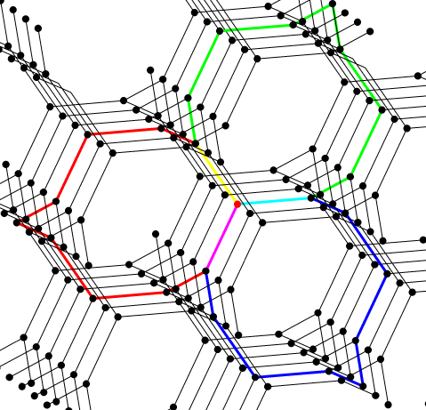
(in a more familiar projection)
on the other hand, that doesnt’ seem a good strategy for extending further.
I’ll continue my studies of the 5-dimensional crystal that’s a universal abelian cover of the cube graph, picking up where I left off.
Instead of trying to compute the density of this crystal, I’ll try to understand a bit about what it “looks like”.
There are 6 kinds of vertices, corresponding to the 6 vertices of the cube. Let’s take a vertex and study the 3 edges coming out of it!
We have direct access to the cube’s 6 faces, which are called 1,2,3,4,5,6. Faces 1 and 2 are diametrically opposite to each other, as are faces 3 and 4, as are faces 5 and 6.
So, there’s a unique vertex incident to faces 1, 3 and 5. Let’s look at that. If I’m getting my signs correct, the 3 edges coming out of this vertex are and
and  . I am probably choosing some sign convention by saying this, and that makes me nervous, but I doubt it will get me in trouble in this little calculation. I’d run a bigger risk if I started studying more than one vertex; then my sign convention would need to be consistent somehow.
Charging boldly ahead:
This was not very thrilling, but we’ve learned that this vertex — hence by symmetry every vertex — has 3 edges coming out of it that are all at this angle to each other:
This is actually interesting. The triamond, obtained by the very same general recipe starting with a tetrahedron rather than a cube, also has 3 edges coming out of each vertex that are at angles to each other.
If I had more energy I would instantly repeat this calculation for the octahedron, dodecahedron and icosahedron.
With our recipe, any trivalent vertex will have its incident edges at to each other, because the edge vectors obey Kirchhoff’s law, and using a regular simplex for the mesh currents means that all edge vectors are of the same length.
The only way three equal-length vectors can sum to zero (i.e. obey Kirchhoff’s law at the vertex) is if they make a symmetrical 3-pointed star like that. So you don’t need to calculate anything to know that the dodecahedron vertices will look the same.
We ought to be able to predict the local configuration at the 4-valent and 5-valent vertices as well. I’d be surprised if the neighbouring vertices in these cases don’t form a regular tetrahedron and a regular 4-simplex, respectively, centred on the starting vertex, since these are the least degenerate possibilities consistent with Kirchhoff’s law and equal-length edge vectors. Of course, it would also be consistent if they formed 4-pointed and 5-pointed stars in a plane, but my hunch is that they don’t.
For the octahedron it’s actually more complicated: two edges on the same face form an angle of 120 degrees, but two edges that aren’t from the same face are actually perpendicular!
Think simple roots of plus minus the sum of those roots.
*along with minus the sum of those roots
Greg wrote:
Okay, great! Boring calculations often reveal results that can be obtained faster by thinking clearly. But I’m still glad I did the boring calculations, because it makes everything seem more ‘real’.
That sounds nice! If so, when we form a highly symmetrical graph by triangulating Klein’s quartic curve with 7 triangles meeting at each corner, in the resulting ‘crystal’ each atom should have 7 neighbors lying at the vertices of a regular 6-simplex. That would be quite pretty!
And so on: we can get lots of crystals like this using surfaces of higher genus.
I’m thinking of calling these Platonic crystals, unless someone has a better name.
Alas, my hunch was wrong; as Layra points out, the symmetry between the edges is broken at the vertices of an octahedron (or icosahedron), because a pair of edges incident on the vertex might or might not belong to the same face.
Yes, I figured it out too while watching TV. If you trace out a loop around the corners of an equilateral triangle, the differences between successive corners are vectors that are themselves the corners of an equilateral triangle. But this pattern fails when we go to a tetrahedron or any higher-dimensional simplex!
It’s related to how
only for
Using John’s construction for the mesh currents forming a regular simplex, and slightly tweaking some of the edge-labelling conventions, wlog we can take the outgoing edge vectors at any vertex in a graph with faces to be, in cyclic order around the vertex:
…
So, cyclically adjacent pairs of edges in the original graph will lift to edges at 120 degrees to each other in the covering graph, and all other pairs of edges at the vertex will lift to mutually perpendicular edges in the covering graph.
Isn’t that last vector supposed to be
That’s very nice. For one thing, if you normalize the vectors you listed to have length squared 2, they have exactly the inner products that you need for the root vectors of the affine Dynkin diagram
I’m not sure exactly what this implies, but affine Dynkin diagrams are to groups generated by reflections and translations as ordinary Coxeter–Dynkin diagrams are to groups generated by reflections (Coxeter groups). So, just as ordinary Coxeter–Dynkin diagrams are a nice way to describe the symmetry groups of Platonic solids, affine Dynkin diagrams are a nice way to describe symmetry groups of very symmetrical lattices. Since each of our ‘Platonic crystals’ has (at least) the lattice as translational symmetries, it’s not shocking to see the
  affine Dynkin diagram show up.
However, I still don’t see quite why it’s showing up in the way it is.
I’m not really sure how relevant the Dynkin connection is, actually. We get for the case of 1-skeleta of polyhedra, but we can easily extend the construction to the 1-skeleton of higher-dimensional polytopes: each face gets assigned a vector and an orientation, directed edges get assigned vectors based on adjacent faces. For the 4-simplex we get angles of arccos(-1/3). So I think the
  connection may be a low-dimensional coincidence.
John wrote:
No, because these are vectors in , where
  is the number of faces in the graph. You’re working in the subspace of dimension
  where the coordinates sum to zero. But there won’t be
  faces around any given vertex, there will be a smaller number, so the list of edge vectors won’t get as far as:
I should have stressed that the length of that list of vectors isn’t , but
, but  , the number of faces incident on some vertex.
Concretely, the point of that block of zeroes remaining at the end of every vector in the list is just that the edge vectors at each vertex don’t generate a full-dimensional sublattice of the lattice spanned by the mesh currents; they generate a lower-dimensional sublattice that is a scaled copy of .
.
Oh, right. I get it.
By the way, I spotted an issue that I haven’t thought about hard enough. I said that choosing face vectors that sum to zero is enough to ensure Kirchhoff’s current law for the edge vectors. That’s definitely true if our graph is drawn on a sphere, but
if it’s drawn on a surface of higher genus I need to be a bit more careful than I have so far!
Actually, right this second I’m leaning toward the opinion that everything is fine. On a surface of higher genus we can have current flowing around a handle, but as long as the surface is connected it seems the number of independent Kirchhoff’s current law constraints equals the number of faces minus 1.
John wrote:
I agreed to that when you said it … but I now think it’s not a necessary condition for satisfying Kirchhoff’s law, regardless of whether the graph is embedded on a sphere or a surface of higher genus. (Of course we do have other, geometrical reasons to want the mesh currents to sum to zero!)
So long as we can put an orientation on every face, we can specify a mesh current for each face and think of that current as flowing around just inside the boundary of the face. It’s easier to think clearly about what’s happening if we pretend for the moment that the mesh currents are scalar parameters, and the geometry of the situation turns them into directional currents moving along the surface in a particular way. So these scalars parameterise conserved vector fields on the surface in which we’ve embedded the graph, and in the idealisation where the currents get ever closer to the border of each face, the field is only non-zero on the edges, and is tangent to the edge.
We can then ascribe to each edge a current that is the vector sum of the mesh currents running along that edge from the two faces incident on the edge. I think this makes things clearer than having to think about choosing an orientation for every edge and worrying about which face’s mesh current we subtract from which at each particular edge.
I believe it’s obvious, then, that the sum of edge currents at any vertex will automatically be zero, because at each vertex, every face’s mesh current will appear twice with opposite signs: once flowing into the vertex and once flowing out of the vertex.
In effect, the whole idea of a conserved current circulating around the border of each face guarantees conservation everywhere: you can’t get any sources or sinks appearing when all you’re really doing is adding up a whole lot of loops!
I should add a remark that reconciles what I said here with some linear-algebraic facts that seem to contradict it, but really don’t!
In the example of the cube, we have 6 faces, 8 vertices and 12 edges. If you choose an orientation on each edge so you can talk about 12 edge current variables , then the system of 8 linear equations that says Kirchhoff’s current law is obeyed at all 8 vertices has rank 7, i.e. one of the equations follows automatically from all the others being true.
So, the solution space in the edge current variables has dimension . Since that’s one less than the number of faces, 6, it seems intuitively obvious that we will need to impose some condition on the 6 mesh currents in order to stay in that 5-dimensional solution space.
But that intuition is wrong! The map from the 6-dimensional space of mesh currents to the space of edge currents is not of maximal rank: it takes the whole 6-dimensional domain into the 5-dimensional subspace of edge currents satisfying Kirchhoff’s current law at every vertex.
BTW, I gather from the Wikipedia article on mesh analysis that when the technique is used to analyse planar circuits, mesh currents are specified only for the loops in the circuit that do not contain any other loop, which in our setup on a sphere would correspond to specifying them for every face of the polygon except one, i.e. setting one face’s mesh current to zero.
That choice makes sense when you’re solving for the currents in a circuit, because it gives you the correct number of parameters and makes the equations as sparse as possible. It would be pointless to add another mesh current around the outside of a planar circuit just to make the sum of all mesh currents equal to zero.
But our choice of making the sum of all mesh currents equal to zero is just as valid in terms of satisfying Kirchhoff’s current law, and for our purposes it makes the geometry much more symmetrical.
Greg wrote:
By the way: for some reason, even though I always knew the opposite edges of a regular tetrahedron are at right angles to each other, I didn’t notice the obvious generalization! If we take a round tour of a higher-dimensional regular simplex, visiting each vertex just once, each edge we traverse will be orthogonal to all the rest, except for the edges that came immediately before and immediately after.
Where did this blindness come from? Maybe it’s because some edges of the regular tetrahedron look orthogonal when you project them down to the plane this way:
whereas no edges look orthogonal in the usual projection of the 4-simplex:
In 4-space, each edge of the outer pentagon is orthogonal to all the others—except for its neighbors, which it meets at a 60° angle. Ditto for the inner pentagram!
Indeed, any two edges in a regular n-simplex either share a vertex, in which case they meet at 60 degrees, or are skew and thus determine a regular tetrahedron, in which case they’re perpendicular.
Yes, it’s one of those things that’s obvious if you think about it. But I’d been dealing with 4-simplexes a lot in my work on quantum gravity, and a lot more since, and I’d never thought about it! I want to spare others my years of benighted ignorance.
Thanks for clarifying this stuff! I was sort of confused.
The study of mesh currents, Kirchhoff’s laws and such is actually what mathematicians would call part of ‘homology theory’, and if/when I write this up more carefully I’ll probably use that way of thinking to debug my brain, but I haven’t really done it yet. In some ways homology theory is overkill, but it’s just right for formalizing the concept of the ‘universal abelian cover’ of a graph, and one thing I want to do someday is carefully prove we’re getting universal abelian covers.
Thank you, John. Interesting as always.
Glad you liked it!
I’ve decided that the lattice generated by edge vectors is more relevant to crystallography than the lattice
  generated by face vectors, since it’s the edge vectors that describe the separations between atoms joined by bonds. In other words, you can take vectors pointing along all the bonds of your crystal, let them generate a lattice, and you get
  It’s harder—at least for me—to look at a crystal and read off the lattice
But I’m getting confused about the relation between these lattices, even when we assume (as we’re usually doing) that the face vectors sum to zero.
We have one face vector for each face
  which are linearly independent except for one constraint: they sum to zero.
From these we define edge vectors
where are the two faces meeting along the edge
  .
.
So, obviously is contained in
  It only knows about differences of face vectors, but that’s so bad, since the sum of all face vectors is zero.
Hmm, right now I’m thinking that is of index
  in
in  . In other words,
Does that seem right?
We’ve also got the lattice generated by loop vectors, which I’ll call . This lattice, unlike the other two, acts as translational symmetries on the set
  of atoms of our crystal. We have
It is fairly easy to see that
the number of vertices in our graph. This says that one atom of each ‘color’ (with the vertices of our graph giving ‘colors’) appears in each unit cell of
Greg proved that
where the right side is the product of nonzero eigenvalues of the Laplacian of the dual graph, and is one less than the number of vertices of the dual graph, or faces of our original graph:
Kirchhoff’s matrix tree theorem says that
where is the number of spanning trees in the dual graph. Putting together the last 3 equations, we get
I should do an example or two to check all this. Indeed, I want to work out the relevant numbers for all the Platonic examples.
So, let me try the example of the degenerate Platonic solid called the ‘trigonal hosohedron’:
This gives the crystal structure of graphene:
or in other words, the hexagonal tiling:
There are two ‘colors’ of atoms here: those with bond poking out to the left and those with a bond poking out to the right. This is because the trigonal hosohedron has two vertices:
The lattice of edge vectors looks like a triangular tiling:
The vertices of the hexagonal tiling occupy only 2/3 of the vertices in the triangular tiling. I had to draw a lot of pictures before I was sure of this simple fact, but now it seems obvious. Mathematically this means
Combining this with the previous equation we get
Continuing with the trigonal hosohedron, I want to check my guess
In this case we have 3 face vectors, say obeying
  These generate the lattice
The sublattice is generated by the differences
  or indeed any two of these.
If we use the equation to eliminate
 is generated by
then
while is generated by
Thus, the index of in
in  is
is
In other words,
which is consistent with my guess
I also want to check Greg’s formula
On the one hand, the trigonal hosohedron has 3 faces, and its dual graph has 3 spanning trees:
so his formula gives
But we can also calculate this quantity in a different way! Since we have
we have
and above I’ve shown
This gives
consistent with Greg’s formula.
This is exciting, because I made some mistakes en route, but now things are working.
Given all this, I can calculate one thing I’m interested in now, which is: “what fraction of the potential locations for atoms in the hexagonal lattice are actually occupied by atoms?” Or in short: what is the packing fraction?
I calculated this density earlier for graphene, but the basic idea is just that graphene has some obvious ‘holes’ where atoms could have been, and the fraction of potential locations that are ‘filled’ is 2/3:
Let’s see how to calculate this systematically starting from the graph that gives rise to this crystal: the trigonal hosohedron.
Mathematically is the set of actual atoms, while
  is the lattice of potential locations for atoms. So, we can define the packing fraction by
The numerator is easy to compute; I’ve argued above that it’s the number of vertices of our graph (here the trigonal hosohedron):
The denominator is tougher; I think we need to use
and solve for the quantity we want:
Then we can use Greg’s result
and my guess
to get
Hey, that’s nice!
So, using Greg’s result and my guess, the packing fraction is:
Nice!
We can check this for the hexagonal lattice. The trigonal hosohedron has 2 vertices, and its dual graph has 3 spanning trees, so we get 2/3, just as we should!
Now let me try a harder example: the dodecahedron!
This gives a crystal in 11 dimensions with 20 different colors of atoms, since the dodecahedron has 12 faces and 20 vertices.
The packing fraction, defined as
is 20 divided by the number of spanning trees in the dual graph, which is the icosahedral graph. Here’s a typical spanning tree in the icosahedral graph:
I got this picture from a Matlab page about a program that counts spanning trees. This page says the icosahedral graph has 5,184,000 spanning trees! So, the density of our 11-dimensional crystal is
It seems the only thing that’s hard to compute is the number of spanning trees. Surely someone has done this for all the Platonic solids!
Great stuff!
I get the following results:
where is the packing fraction relative to the edge vector lattice and
  is the number of spanning trees of the dual graph. I computed
  from the graph Laplacian.
This all fits in with your conjecture that the index of the edge vector lattice in the face vector lattice is , which shouldn’t be too hard to prove.
It’s interesting how seems to be the same for the dual when the graph embeds into the sphere, but not for higher genus.
Thanks a million! I assume your here is what I’m now calling the packing fraction, not the quantity you used to call
  (It must be, because your results match mine.)
While you’re doing these, could you please also do two more? The cuboctahedron:
and the icosidodecahedron:
are nice because their symmetry groups acts transitively on their vertex-edge flags. I believe this implies the associated crystal also has a symmetry group acting transitively on the vertex-edge flags. Sunada calls such crystals strongly isotropic, and he raised the challenge of classifying them. One of the best things about the Platonic crystals is that they’re strongly isotropic, but those coming from the cuboctahedron and icosidodecahedron are equally good in this respect (as are those coming from Klein’s quartic curve and infinitely many other highly symmetric tilings of higher-genus surfaces).
I don’t know if I’ve found all graphs embedded in the sphere that have symmetry groups that act transitively on flags!
Yes, here is the packing fraction relative to the edge vector lattice (not the face vector lattice).
For those other polyhedra:
Oh, I see that it’s a well-known result that, for planar graphs, the graph and its dual have the same number of spanning trees.
Wow, the proof is so beautiful I have to quote it:
This reminds me a lot of the Hodge star operator on a surface.
The discrete analogue of a 1-form on a surface is a 1-cochain, i.e. a function assigning a number to each directed edge in a polygonal decomposition of that surface. The ‘Hodge dual’ of a 1-cochain is the 1-cochain on the dual graph, which assigns to each dual edge the same number that the original 1-cochain assigned to the corresponding edge on the original graph.
I’d hope that following this analogy, we’d get some direct way to see why the product of nonzero eigenvalues of the Laplacian on a graph on the sphere equals the product of nonzero eigenvalues of the Laplacian on the dual graph! This fact follows from the fact you just mentioned together with Kirchhoff’s matrix tree theorem. But it should have some proof based on the relation between cochains on a graph and cochains on the dual graph.
Here’s a sketch of a proof that the index of the edge vector lattice in the face vector lattice
  is
is  , when the face vectors sum to zero. I’ll illustrate it with the cube as an example, so
  .
.
If the face vectors lie in , and the edge vectors are all differences of pairs of face vectors, then in terms of the
  face vectors, the
  coefficients of any edge vector are integer-linear combinations of the
  rows of a matrix like this:
For any pair of face vectors involving only the first faces, we can take the difference of two of these rows to obtain the edge vector, and for any pair that includes the last face, the edge vector is simply one of these rows as it stands (or its opposite). So we can certainly obtain any edge vector this way.
Conversely, we can obtain any row of this matrix as an integer-linear combination of edge vectors, by finding a path through the dual graph from the last face to the face whose number is the row number and summing the edge vectors (or their opposites) for the edges dual to those in the path. All the face vectors we pass through can be cancelled out, leaving only those at the start and end of the path.
Next, we need to account for the fact that the face vectors aren’t linearly independent, and rewrite this matrix replacing the last face vector with minus the sum of all the others. We then obtain a matrix like this:
All we’ve done here is add 1 to every entry and drop the last column, since we are subtracting the vector:
rather than including the in the last column.
The sum of all the rows of will be the same in every column: one more than the number of rows. Since the number of rows is
  , the sum of the rows will be:
We don’t change the determinant of if we add every other row to the last row to turn it into that sum, and then, we don’t change the determinant by subtracting that new last row, divided by
  , from every other row. This removes the effect of adding 1 to all the entries that took us from
  to
to  , for the first
  rows, so we reach a matrix that agrees with
  for the first
  rows and
  columns, and ends with the row:
For our example of the cube:
So we have .
.
Excellent! I arrived at my guess via some manipulations roughly like this, but in the case of the tetrahedron, so that generalizing it seemed a bit tricky. For the tetrahedron, all those paths you mention have length 1, so it was hard to recognize them as paths!
We’ve seen that for graphs drawn on a surface, Kirchhoff’s matrix tree theorem is equivalent to a simple formula for the number of points in the quotient : it’s the number of spanning trees in the dual graph.
Note that while we’ve been using ‘face vectors’ to get ‘edge vectors’ and then ‘loop vectors’, all the counting we’ve been doing in the last 6 or 7 comments didn’t depend on what those face vectors were.
And indeed, the lattice of loop vectors has a nice meaning independent of our choice of face vectors: it’s isomorphic to the first homology group
  of our graph
I believe the lattice of edge vectors has a similar abstract interpretation: it’s some sort of subgroup or quotient group of the free abelian group on the set of edges. The free abelian group on the set of edges is usually called the group of 1-chains and denoted
If I could figure out this abstract interpretation, I’d have a nice highbrow statement of Kirchhoff’s matrix tree theorem! The first homology group of a graph (namely ) sits inside some bigger free abelian group that we can get from a graph (namely
  ) and the number of points in the quotient is the number of spanning trees in the dual graph.
And if our original graph is planar, that’s also the number of spanning trees in our original graph! It might even give a clearer way to understand Kirchhoff’s matrix tree theorem. Ideally, there’d be a natural bijection between spanning trees and points in
Probably someone has already figured out most of this, indeed it’s probably in Sunada’s book Topological Cystallography, but I want to understand it.
For a second I thought the lattice of edge vectors was itself isomorphic to but of course it’s not, because the lattice of edge vectors has a smaller rank.
  is a free abelian group with as many generatores as edges of our graph, while
  is a free abelian group with as many generators as independent loops of our graph.
Sunada has a somewhat different abstract interpretation of Kirchhoff’s matrix tree theorem. It’s Theorem 10.8 in his book Topological Crystallography, though he may not have been the first to prove it.
He starts with a graph and lets
  consist of functions from vertices of
  to
to  with the property that when you sum their values over all vertices you get zero.
where is the graph Laplacian. Let’s call this subgroup
He shows that the number of points of is the number of spanning trees in
Note that this ‘summing over all vertices gives zero’ condition is dual to our condition on face vectors, where we like the sum over all faces to give zero. Note also that his formulation doesn’t mention the dual graph of So apparently he has moved completely over to the dual picture, as compared to us.
And also somehow he’s managing to talk about “0-cochains” (functions from vertices to ) instead of “1-chains” (integer linear combinations of edges).
• P. Bacher, P. de la Harpe and T. Nagnibeda, The lattice of integral flows and the lattice of integral cuts, Bull. Soc. Math. France 125 (2) (1997), 167–198.
Might be helpful if you haven’t seen it.
Thanks! I believe they proved some of the stuff Greg just proved, and more generally.
Namely, for any finite directed graph they let the space of 1-cochains
  consist of functions from edges to integers. This is isomorphic to the lattice I’ve been calling
  : the lattice spanned by ‘edge vectors’.
They define a Laplacian on 1-cochains: given a 1-cochain
  they define
  to be
to be  , minus the sum of
  over edges
  that end where
  starts, minus the sum of
  over edges
  that start where
  ends.
ends.
They let consist of 1-cochains that are in the kernel of the Laplacian. This is isomorphic to the lattice that I’ve recently taken to calling
  : the lattice spanned by ‘loop vectors’.
Greg and I showed that
where is the number of spanning trees in the graph.
I believe their Proposition 1.3 is closely related to this result. They say:
The complexity of is just the number of spanning trees.
Hmm, but I’m a bit puzzled about this ‘determinant’.
I’ve just realised that some of the results we’ve proved won’t hold for graphs that embed in surfaces of higher genus, such as Klein’s quartic curve. So, those packing densities I calculated for the two graphs in Klein’s quartic curve are almost certainly wrong.
I computed a basis for the lattice of translation symmetries of the crystal by assuming that you get a basis for all the loops in the graph by following the edges around each of
  faces. But the dimension of the cycle space of a graph is always
  for a graph with
  connected components. For a single connected component, we have:
where is the Euler characteristic. For a sphere
  and the dimension of the cycle space is
  , but for Klein’s quartic curve with
  , we have
  .
.
This means that for a graph embedded in Klein’s quartic curve, there will be loops in the graph such that when we sum the associated edge vectors, the result need not lie in the lattice generated by the vectors we get from taking loops around all but one face in the graph. I say “need not” rather than “does not”, because if we’re still working in there’s the complication that the full set of
  loop vectors won’t be linearly independent, so I’m not sure exactly what will happen. The one thing that’s clear is that all integer-linear combinations of all
  loop vectors will yield translation symmetries of the crystal, whether or not that lattice in
  is the same as the one generated by the
  loops associated with faces.
You’re right. For each extra handle you add to a torus, you get two noncontractible loops that cross each other: one that runs ‘around’ the handle and one that runs ‘along’ it. (Sorry, those prepositions quite don’t do justice to the geometry.) So for Klein’s quartic we must take into account 6 loops besides the ones that run around faces.
The fancy way to talk about this relates the first homology group of the graph (which is a free abelian group on some number of generators) to the first homology group of the surface (which is a free abelian group on some smaller number of generators).
[…] I read an interesting blog post by a mathematician, John Baez, on the structure of diamonds and triamonds. […]
A while back, we started talking about crystals:
• John Baez, Diamonds and triamonds, Azimuth, 11 April 2016.
In the comments on that post, a bunch of us worked on some puzzles connected to ‘topological crystallography’—a subject that blends graph theory, topology and mathematical crystallography. You can learn more about that subject here:
• Tosio Sunada, Crystals that nature might miss creating, Notices of the AMS 55 (2008), 208–215.
Greg Egan and I got so interested that we wrote a paper about it!
• John Baez and Greg Egan, Topological crystals.
A lot of different diamondoids occur naturally in petroleum. Though the carbon in diamonds is not biological in origin, the diamondoids found in petroleum are composed of carbon from biological sources. This was shown by studying the ratios of carbon isotopes present.
Eric Drexler has proposed using diamondoids for nanotechnology, but he’s talking about larger molecules than those shown here.
For more fun along these lines, try:
• Diamonds and triamonds, Azimuth, 11 April 2016.
[…] John Baez elaborates on the sequence of ‘hyperdiamonds’, together with mentioning an alternative three-dimensional structure called the triamond, here. […]