
Last time I explained how to create the ‘maximal abelian cover’ of a connected graph. Now I’ll say more about a systematic procedure for embedding this into a vector space. That will give us a topological crystal, like the one above.
Some remarkably symmetrical patterns arise this way! For example, starting from this graph:
we get this:

Nature uses this pattern for crystals of graphene.
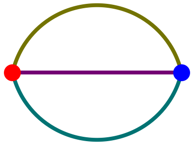
Starting from this graph:

we get this:

Nature uses this for crystals of diamond! Since the construction depends only on the topology of the graph we start with, we call this embedded copy of its maximal abelian cover a topological crystal.
Today I’ll remind you how this construction works. I’ll also outline a proof that it gives an embedding of the maximal abelian cover if and only if the graph has no bridges: that is, edges that disconnect the graph when removed. I’ll skip all the hard steps of the proof, but they can be found here:
• John Baez, Topological crystals.
The homology of graphs
I’ll start with some standard stuff that’s good to know. Let 


The group of integral 0-chains on 


such that
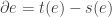
for each edge

is the group of integral 1-cycles on
Remember, a path in a graph is a sequence of edges, the target of each one being the source of the next. Any path 

For any path 

and if 

Last time I explained what it means for two paths to be ‘homologous’. Here’s the quick way to say it. There’s groupoid called the fundamental groupoid of 

![[[\gamma]] : x \to y](https://s0.wp.com/latex.php?latex=%5B%5B%5Cgamma%5D%5D+%3A+x+%5Cto+y&bg=ffffff&fg=333333&s=0&c=20201002)

![[[\gamma]] = [[\gamma']]](https://s0.wp.com/latex.php?latex=%5B%5B%5Cgamma%5D%5D+%3D+%5B%5B%5Cgamma%27%5D%5D&bg=ffffff&fg=333333&s=0&c=20201002)
Here’s a nice thing:
Lemma A. Let 

Proof. See the paper. You could say they give ‘homologous’ 1-chains, too, but for graphs that’s the same as being equal. █
We define vector spaces of 0-chains and 1-chains by

respectively. We extend the boundary map to a linear map

We let 

and we call elements of this vector space 1-cycles. Since 


This is the key to building topological crystals!
The embedding of atoms
We now come to the main construction, first introduced by Kotani and Sunada. To build a topological crystal, we start with a connected graph 
![[[\alpha]] : x_0 \to x](https://s0.wp.com/latex.php?latex=%5B%5B%5Calpha%5D%5D+%3A+x_0+%5Cto+x++&bg=ffffff&fg=333333&s=0&c=20201002)
Last time I showed that these atoms are the vertices of the maximal abelian cover of
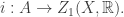
Definition. Let 

by
![i([[ \alpha ]]) = \pi(c_\alpha) .](https://s0.wp.com/latex.php?latex=i%28%5B%5B+%5Calpha+%5D%5D%29+%3D+%5Cpi%28c_%5Calpha%29+.&bg=ffffff&fg=333333&s=0&c=20201002)
That 
Theorem A. The following are equivalent:
(1) The graph
(2) The map 
Proof. The map ![[[ \alpha ]]](https://s0.wp.com/latex.php?latex=%5B%5B+%5Calpha+%5D%5D&bg=ffffff&fg=333333&s=0&c=20201002)
![[[ \beta ]]](https://s0.wp.com/latex.php?latex=%5B%5B+%5Cbeta+%5D%5D&bg=ffffff&fg=333333&s=0&c=20201002)
![i([[ \alpha ]]) = i([[ \beta ]])](https://s0.wp.com/latex.php?latex=i%28%5B%5B+%5Calpha+%5D%5D%29++%3D+i%28%5B%5B+%5Cbeta+%5D%5D%29&bg=ffffff&fg=333333&s=0&c=20201002)
![[[ \alpha ]]= [[ \beta ]]](https://s0.wp.com/latex.php?latex=%5B%5B+%5Calpha+%5D%5D%3D+%5B%5B+%5Cbeta+%5D%5D&bg=ffffff&fg=333333&s=0&c=20201002)


![\pi(c_\gamma) = \pi(c_{\alpha} - c_\beta) = i([[ \alpha ]]) - i([[ \beta ]])](https://s0.wp.com/latex.php?latex=%5Cpi%28c_%5Cgamma%29+%3D+%5Cpi%28c_%7B%5Calpha%7D+-+c_%5Cbeta%29+%3D++i%28%5B%5B+%5Calpha+%5D%5D%29+-+i%28%5B%5B+%5Cbeta+%5D%5D%29+&bg=ffffff&fg=333333&s=0&c=20201002)
Since 

![c_{\gamma} \textrm{ is orthogonal to every 1-cycle} \; \iff \; i([[ \alpha ]]) = i([[ \beta ]])](https://s0.wp.com/latex.php?latex=c_%7B%5Cgamma%7D+%5Ctextrm%7B+is+orthogonal+to+every+1-cycle%7D+++%5C%3B+%5Ciff+%5C%3B+++i%28%5B%5B+%5Calpha+%5D%5D%29++%3D+i%28%5B%5B+%5Cbeta+%5D%5D%29++++&bg=ffffff&fg=333333&s=0&c=20201002)
On the other hand, Lemma A says
![c_\gamma = 0 \; \iff \; [[ \alpha ]]= [[ \beta ]].](https://s0.wp.com/latex.php?latex=c_%5Cgamma+%3D+0+%5C%3B+%5Ciff+%5C%3B+%5B%5B+%5Calpha+%5D%5D%3D+%5B%5B+%5Cbeta+%5D%5D.&bg=ffffff&fg=333333&s=0&c=20201002)
Thus, to prove (1)


The following lemmas are the key to the theorem above — and also a deeper one saying that if
For now, we just need to show that any nonzero 1-chain coming from a path in a bridgeless graph has nonzero inner product with some 1-cycle. The following lemmas, inspired by an idea of Ilya Bogdanov, yield an algorithm for actually constructing such a 1-cycle. This 1-cycle also has other desirable properties, which will come in handy later.
To state these, let a simple path be one in which each vertex appears at most once. Let a simple loop be a loop 


Thus,
Okay, here are the lemmas!
Lemma B. Let 

where 

Proof. See the paper. The proof is an algorithm that builds a simple loop 


Lemma C. Let 


where 

Proof. This relies on the previous lemma, and the proof is similar — but when we can’t subtract off any more 
Lemma D. Let
(1)
(2) For any path 
Proof. It’s easy to show a bridge 

Then, assuming 


I’m deliberately glossing over some difficulties that can arise, so see the paper for details! █
Embedding the whole crystal
Okay: so far, we’ve taken a connected bridgeless graph
These atoms are the vertices of the maximal abelian cover 

The idea is that just as 
Theorem B. If 

sending each edge of
Proof. The first part is easy; the second part takes real work! The problem is to show the edges don’t cross. Greg Egan and I couldn’t do it using just Lemma D above. However, there’s a nice argument that goes back and uses Lemma C — read the paper for details.
As usual, history is different than what you read in math papers: David Speyer gave us a nice proof of Lemma D, and that was good enough to prove that atoms are mapped into the space of 1-cycles in a one-to-one way, but we only came up with Lemma C after weeks of struggling to prove the edges don’t cross. █
Connections to tropical geometry
Tropical geometry sets up a nice analogy between Riemann surfaces and graphs. The Abel–Jacobi map embeds any Riemann surface 


After I put this paper on the arXiv, I got an email from Matt Baker saying that he had already proved Theorem A — or to be precise, something that’s clearly equivalent. It’s Theorem 1.8 here:
• Matthew Baker and Serguei Norine, Riemann–Roch and Abel–Jacobi theory on a finite graph.
This says that the vertices of a bridgeless graph
What I really want to know is whether someone’s written up a proof that this map embeds the whole graph, not just its vertices, into its Jacobian in a one-to-one way. That would imply Theorem B. For more on this, try my conversation with David Speyer.
Anyway, there’s a nice connection between topological crystallography and tropical geometry, and not enough communication between the two communities. Once I figure out what the tropical folks have proved, I will revise my paper to take that into account.
Next time I’ll talk about more examples of topological crystals!
Read the whole series
• Part 1 – the basic idea.
• Part 2 – the maximal abelian cover of a graph.
• Part 3 – constructing topological crystals.
• Part 4 – examples of topological crystals.


Dear John. I am excited about the links with tropical geometry. Tropical geometry and non-archimedean mathematics are something I would love to touch at my blog (now paused due to some personal and academical issues). I have enjoyed to see tropical connections with graph theory…
To go beyond: What about tropical spacetime physics or tropical Quantum Mechanics? What about a polycrystalline tropically quantum spacetime?
You can combine ideas in many ways, but throwing them together at random is rarely opimtal. Tropical mathematics is really the ‘classical limit’ or ‘low-temperature limit’ of mathematics using complex numbers. I discussed this in weeks 11, 12 and 13 of my Winter 2007 seminar: you can read the notes. I also recommend this:
• Grigori L. Litvinov, The Maslov dequantization, idempotent and tropical mathematics: a very brief introduction.
I think this is the most promising way to apply tropical mathematics to physics.
OH, I did not remember that! You have been so prolific than I forgot your QG seminar touching this fascinating topic. What about a p-adic/tropical geometry dictionary? Does it exist if any? It is interesting your comment about tropical math as the “classical” limit of quantum math. Low temperature physics is purely quantum at nature (e.g., see the BEC phase transition!). Tropical mathematics is yet a young branch but I am sure physisics will face with it much more in the near future.
Interesting…Tropical mathematics as “low T limit of mathematics”. I will reread your winter 2007 seminar…I had almost forgotten it completely! And what about the high temperature limit?
Good puzzle! You can work it out yourself using the formulas on page 18 here.
While I try to digest the maths, on the version I see there’s two repeated sentences on tbe third-last paragraph.
Thanks! I love it when people catch my typos.
Next time I’ll give tons of examples. All this was just to define the construction and prove it gives a “crystal” embedded in a vector space.
Hey, I’d like to go into medicine myself but I was wondering what made you pick maths and physics. Out of interest 😊. It’s just your passion really comes across.
When I was young, I really wanted to understand everything about the universe—and especially the most basic, fundamental things. So, I wanted to start by learning the laws of physics, since these govern everything. As I went further, I realized that the laws of physics are written in the language of mathematics, so I got interested in that.
I also discovered that profound questions like “what is true?” and “how do we know anything?” led people to develop logic. Thanks to a book my dad checked out of the public library, I learned that in the 20th century Gödel and others proved theorems in logic that put limits on what we can prove. So I got interested in logic, which nowadays is another branch of mathematics.
Nowadays I feel I know enough math and physics to start thinking about other things, like global warming, biology, and a general theory of networks. But occasionally I want to work on pure math, so I do projects like this one on topological crystals.
That’s such a great development. Cool.