A Compositional Framework for Reaction Networks

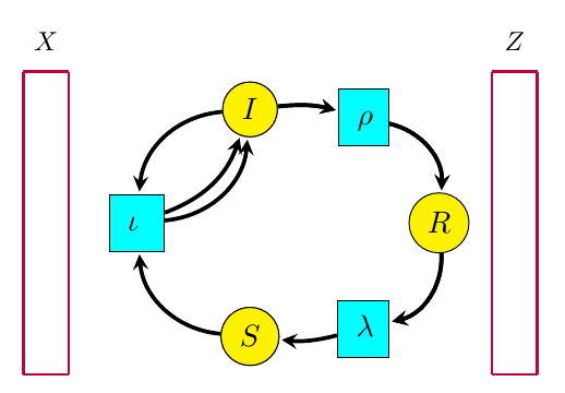
For a long time Blake Pollard and I have been working on ‘open’ chemical reaction networks: that is, networks of chemical reactions where some chemicals can flow in from an outside source, or flow out. The picture to keep in mind is something like this:

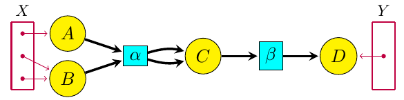
where the yellow circles are different kinds of chemicals and the aqua boxes are different reactions. The purple dots in the sets X and Y are ‘inputs’ and ‘outputs’, where certain kinds of chemicals can flow in or out.

Here’s our paper on this stuff:

• John Baez and Blake Pollard, A compositional framework for reaction networks, Reviews in Mathematical Physics 29 (2017), 1750028.

Blake and I gave talks about this stuff in Luxembourg this June, at a nice conference called Dynamics, thermodynamics and information processing in chemical networks. So, if you’re the sort who prefers talk slides to big scary papers, you can look at those:

• John Baez, The mathematics of open reaction networks.

• Blake Pollard, Black-boxing open reaction networks.

But I want to say here what we do in our paper, because it’s pretty cool, and it took a few years to figure it out. To get things to work, we needed my student Brendan Fong to invent the right category-theoretic formalism: ‘decorated cospans’. But we also had to figure out the right way to think about open dynamical systems!

In the end, we figured out how to first ‘gray-box’ an open reaction network, converting it into an open dynamical system, and then ‘black-box’ it, obtaining the relation between input and output flows and concentrations that holds in steady state. The first step extracts the dynamical behavior of an open reaction network; the second extracts its static behavior. And both these steps are functors!

Lawvere had the idea that the process of assigning ‘meaning’ to expressions could be seen as a functor. This idea has caught on in theoretical computer science: it’s called ‘functorial semantics’. So, what we’re doing here is applying functorial semantics to chemistry.

Now Blake has passed his thesis defense based on this work, and he just needs to polish up his thesis a little before submitting it. This summer he’s doing an internship at the Princeton branch of the engineering firm Siemens. He’s working with Arquimedes Canedo on ‘knowledge representation’.

But I’m still eager to dig deeper into open reaction networks. They’re a small but nontrivial step toward my dream of a mathematics of living systems. My working hypothesis is that living systems seem ‘messy’ to physicists because they operate at a higher level of abstraction. That’s what I’m trying to explore.

Here’s the idea of our paper.

The idea

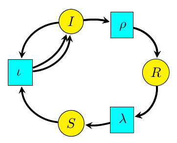
Reaction networks are a very general framework for describing processes where entities interact and transform int other entities. While they first showed up in chemistry, and are often called ‘chemical reaction networks’, they have lots of other applications. For example, a basic model of infectious disease, the ‘SIRS model’, is described by this reaction network:

We see here three types of entity, called species:

• : susceptible,
• : infected,
• : resistant.

We also have three `reactions’:

• : infection, in which a susceptible individual meets an infected one and becomes infected;
• : recovery, in which an infected individual gains resistance to the disease;
• : loss of resistance, in which a resistant individual becomes susceptible.

In general, a reaction network involves a finite set of species, but reactions go between complexes, which are finite linear combinations of these species with natural number coefficients. The reaction network is a directed graph whose vertices are certain complexes and whose edges are called reactions.

If we attach a positive real number called a rate constant to each reaction, a reaction network determines a system of differential equations saying how the concentrations of the species change over time. This system of equations is usually called the rate equation. In the example I just gave, the rate equation is

Here and are the rate constants for the three reactions, and now stand for the concentrations of the three species, which are treated in a continuum approximation as smooth functions of time:

The rate equation can be derived from the law of mass action, which says that any reaction occurs at a rate equal to its rate constant times the product of the concentrations of the species entering it as inputs.

But a reaction network is more than just a stepping-stone to its rate equation! Interesting qualitative properties of the rate equation, like the existence and uniqueness of steady state solutions, can often be determined just by looking at the reaction network, regardless of the rate constants. Results in this direction began with Feinberg and Horn’s work in the 1960’s, leading to the Deficiency Zero and Deficiency One Theorems, and more recently to Craciun’s proof of the Global Attractor Conjecture.

In our paper, Blake and I present a ‘compositional framework’ for reaction networks. In other words, we describe rules for building up reaction networks from smaller pieces, in such a way that its rate equation can be figured out knowing those those of the pieces. But this framework requires that we view reaction networks in a somewhat different way, as ‘Petri nets’.

Petri nets were invented by Carl Petri in 1939, when he was just a teenager, for the purposes of chemistry. Much later, they became popular in theoretical computer science, biology and other fields. A Petri net is a bipartite directed graph: vertices of one kind represent species, vertices of the other kind represent reactions. The edges into a reaction specify which species are inputs to that reaction, while the edges out specify its outputs.

You can easily turn a reaction network into a Petri net and vice versa. For example, the reaction network above translates into this Petri net:

Beware: there are a lot of different names for the same thing, since the terminology comes from several communities. In the Petri net literature, species are called places and reactions are called transitions. In fact, Petri nets are sometimes called ‘place-transition nets’ or ‘P/T nets’. On the other hand, chemists call them ‘species-reaction graphs’ or ‘SR-graphs’. And when each reaction of a Petri net has a rate constant attached to it, it is often called a ‘stochastic Petri net’.

While some qualitative properties of a rate equation can be read off from a reaction network, others are more easily read from the corresponding Petri net. For example, properties of a Petri net can be used to determine whether its rate equation can have multiple steady states.

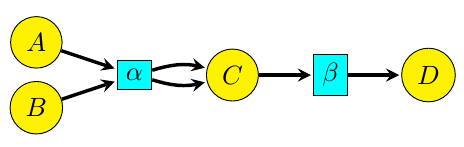
Petri nets are also better suited to a compositional framework. The key new concept is an ‘open’ Petri net. Here’s an example:

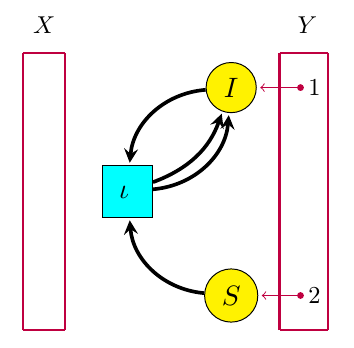
The box at left is a set X of ‘inputs’ (which happens to be empty), while the box at right is a set Y of ‘outputs’. Both inputs and outputs are points at which entities of various species can flow in or out of the Petri net. We say the open Petri net goes from X to Y. In our paper, we show how to treat it as a morphism in a category we call .

Given an open Petri net with rate constants assigned to each reaction, our paper explains how to get its ‘open rate equation’. It’s just the usual rate equation with extra terms describing inflows and outflows. The above example has this open rate equation:

Here are arbitrary smooth functions describing outflows as a function of time.

Given another open Petri net for example this:

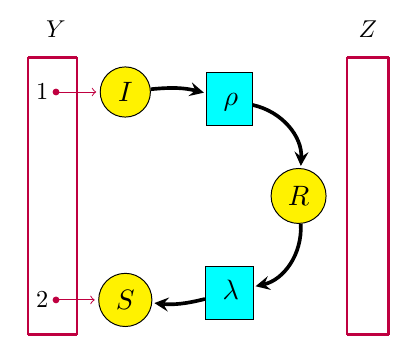
it will have its own open rate equation, in this case

Here are arbitrary smooth functions describing inflows as a function of time. Now for a tiny bit of category theory: we can compose and by gluing the outputs of to the inputs of This gives a new open Petri net as follows:

But this open Petri net has an empty set of inputs, and an empty set of outputs! So it amounts to an ordinary Petri net, and its open rate equation is a rate equation of the usual kind. Indeed, this is the Petri net we have already seen.

As it turns out, there’s a systematic procedure for combining the open rate equations for two open Petri nets to obtain that of their composite. In the example we’re looking at, we just identify the outflows of with the inflows of (setting and ) and then add the right hand sides of their open rate equations.

The first goal of our paper is to precisely describe this procedure, and to prove that it defines a functor

from to a category where the morphisms are ‘open dynamical systems’. By a dynamical system, we essentially mean a vector field on which can be used to define a system of first-order ordinary differential equations in variables. An example is the rate equation of a Petri net. An open dynamical system allows for the possibility of extra terms that are arbitrary functions of time, such as the inflows and outflows in an open rate equation.

In fact, we prove that and are symmetric monoidal categories and that is a symmetric monoidal functor. To do this, we use Brendan Fong’s theory of ‘decorated cospans’.

Decorated cospans are a powerful general tool for describing open systems. A cospan in any category is just a diagram like this:

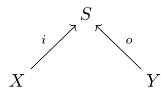
We are mostly interested in cospans in the category of finite sets and functions between these. The set , the so-called apex of the cospan, is the set of states of an open system. The sets and are the inputs and outputs of this system. The legs of the cospan, meaning the morphisms and describe how these inputs and outputs are included in the system. In our application, is the set of species of a Petri net.

For example, we may take this reaction network:

treat it as a Petri net with :

and then turn that into an open Petri net by choosing any finite sets and maps , , for example like this:

(Notice that the maps including the inputs and outputs into the states of the system need not be one-to-one. This is technically useful, but it introduces some subtleties that I don’t feel like explaining right now.)

An open Petri net can thus be seen as a cospan of finite sets whose apex is ‘decorated’ with some extra information, namely a Petri net with as its set of species. Fong’s theory of decorated cospans lets us define a category with open Petri nets as morphisms, with composition given by gluing the outputs of one open Petri net to the inputs of another.

We call the functor

gray-boxing because it hides some but not all the internal details of an open Petri net. (In the paper we draw it as a gray box, but that’s too hard here!)

We can go further and black-box an open dynamical system. This amounts to recording only the relation between input and output variables that must hold in steady state. We prove that black-boxing gives a functor

(yeah, the box here should be black, and in our paper it is). Here is a category where the morphisms are semi-algebraic relations between real vector spaces, meaning relations defined by polynomials and inequalities. This relies on the fact that our dynamical systems involve algebraic vector fields, meaning those whose components are polynomials; more general dynamical systems would give more general relations.

That semi-algebraic relations are closed under composition is a nontrivial fact, a spinoff of the Tarski–Seidenberg theorem. This says that a subset of defined by polynomial equations and inequalities can be projected down onto , and the resulting set is still definable in terms of polynomial identities and inequalities. This wouldn’t be true if we didn’t allow inequalities. It’s neat to see this theorem, important in mathematical logic, showing up in chemistry!

Structure of the paper

Okay, now you’re ready to read our paper! Here’s how it goes:

In Section 2 we review and compare reaction networks and Petri nets. In Section 3 we construct a symmetric monoidal category where an object is a finite set and a morphism is an open reaction network (or more precisely, an isomorphism class of open reaction networks). In Section 4 we enhance this construction to define a symmetric monoidal category where the transitions of the open reaction networks are equipped with rate constants. In Section 5 we explain the open dynamical system associated to an open reaction network, and in Section 6 we construct a symmetric monoidal category of open dynamical systems. In Section 7 we construct the gray-boxing functor

In Section 8 we construct the black-boxing functor

We show both of these are symmetric monoidal functors.

Finally, in Section 9 we fit our results into a larger ‘network of network theories’. This is where various results in various papers I’ve been writing in the last few years start assembling to form a big picture! But this picture needs to grow….