Here’s a draft of a little thing I’m writing for the Newsletter of the London Mathematical Society. The regular icosahedron is connected to many ‘exceptional objects’ in mathematics, and here I describe two ways of using it to construct One uses a subring of the quaternions called the ‘icosians’, while the other uses Patrick du Val’s work on the resolution of Kleinian singularities. I leave it as a challenge to find the connection between these two constructions!
In mathematics, every sufficiently beautiful object is connected to all others. Many exciting adventures, of various levels of difficulty, can be had by following these connections. Take, for example, the icosahedron—that is, the regular icosahedron, one of the five Platonic solids. Starting from this it is just a hop, skip and a jump to the lattice, a wonderful pattern of points in 8 dimensions! As we explore this connection we shall see that it also ties together many other remarkable entities: the golden ratio, the quaternions, the quintic equation, a highly symmetrical 4-dimensional shape called the 600-cell, and a manifold called the Poincaré homology 3-sphere.
Indeed, the main problem with these adventures is knowing where to stop! The story we shall tell is just a snippet of a longer one involving the McKay correspondence and quiver representations. It would be easy to bring in the octonions, exceptional Lie groups, and more. But it can be enjoyed without these esoteric digressions, so let us introduce the protagonists without further ado.
The icosahedron has a long history. According to a comment in Euclid’s Elements it was discovered by Plato’s friend Theaetetus, a geometer who lived from roughly 415 to 369 BC. Since Theaetetus is believed to have classified the Platonic solids, he may have found the icosahedron as part of this project. If so, it is one of the earliest mathematical objects discovered as part of a classification theorem. It’s hard to be sure. In any event, it was known to Plato: in his Timaeus, he argued that water comes in atoms of this shape.
The icosahedron has 20 triangular faces, 30 edges, and 12 vertices. We can take the vertices to be the four points
and all those obtained from these by cyclic permutations of the coordinates, where
is the golden ratio. Thus, we can group the vertices into three orthogonal golden rectangles: rectangles whose proportions are to 1.
In fact, there are five ways to do this. The rotational symmetries of the icosahedron permute these five ways, and any nontrivial rotation gives a nontrivial permutation. The rotational symmetry group of the icosahedron is thus a subgroup of Moreover, this subgroup has 60 elements. After all, any rotation is determined by what it does to a chosen face of the icosahedron: it can map this face to any of the 20 faces, and it can do so in 3 ways. The rotational symmetry group of the icosahedron is therefore a 60-element subgroup of Group theory therefore tells us that it must be the alternating group
The lattice is harder to visualize than the icosahedron, but still easy to characterize. Take a bunch of equal-sized spheres in 8 dimensions. Get as many of these spheres to touch a single sphere as you possibly can. Then, get as many to touch those spheres as you possibly can, and so on. Unlike in 3 dimensions, where there is ‘wiggle room’, you have no choice about how to proceed, except for an overall rotation and translation. The balls will inevitably be centered at points of the lattice!
We can also characterize the lattice as the one giving the densest packing of spheres among all lattices in 8 dimensions. This packing was long suspected to be optimal even among those that do not arise from lattices—but this fact was proved only in 2016, by the young mathematician Maryna Viazovska [V].
We can also describe the lattice more explicitly. In suitable coordinates, it consists of vectors for which:
1) the components are either all integers or all integers plus and
2) the components sum to an even number.
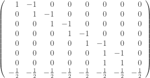
This lattice consists of all integral linear combinations of the 8 rows of this matrix:
The inner product of any row vector with itself is 2, while the inner product of distinct row vectors is either 0 or -1. Thus, any two of these vectors lie at an angle of either 90° or 120°. If we draw a dot for each vector, and connect two dots by an edge when the angle between their vectors is 120° we get this pattern:
This is called the Dynkin diagram. In the first part of our story we shall find the lattice hiding in the icosahedron; in the second part, we shall find this diagram. The two parts of this story must be related—but the relation remains mysterious, at least to me.
The Icosians
The quickest route from the icosahedron to goes through the fourth dimension. The symmetries of the icosahedron can be described using certain quaternions; the integer linear combinations of these form a subring of the quaternions called the ‘icosians’, but the icosians can be reinterpreted as a lattice in 8 dimensions, and this is the lattice [CS]. Let us see how this works.
The quaternions, discovered by Hamilton, are a 4-dimensional algebra
with multiplication given as follows:
It is a normed division algebra, meaning that the norm
obeys
for all The unit sphere in is thus a group, often called because its elements can be identified with unitary matrices with determinant 1. This group acts as rotations of 3-dimensional Euclidean space, since we can see any point in as a purely imaginary quaternion and the quaternion is then purely imaginary for any Indeed, this action gives a double cover
where is the group of rotations of
We can thus take any Platonic solid, look at its group of rotational symmetries, get a subgroup of and take its double cover in If we do this starting with the icosahedron, we see that the 60-element group is covered by a 120-element group called the binary icosahedral group.
The elements of are quaternions of norm one, and it turns out that they are the vertices of a 4-dimensional regular polytope: a 4-dimensional cousin of the Platonic solids. It deserves to be called the “hypericosahedron”, but it is usually called the 600-cell, since it has 600 tetrahedral faces. Here is the 600-cell projected down to 3 dimensions, drawn using Robert Webb’s Stella software:
Explicitly, if we identify with the elements of are the points
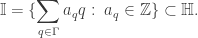
and those obtained from these by even permutations of the coordinates. Since these points are closed under multiplication, if we take integral linear combinations of them we get a subring of the quaternions:
Conway and Sloane [CS] call this the ring of icosians. The icosians are not a lattice in the quaternions: they are dense. However, any icosian is of the form where and live in the golden field
Thus we can think of an icosian as an 8-tuple of rational numbers. Such 8-tuples form a lattice in 8 dimensions.
In fact we can put a norm on the icosians as follows. For the usual quaternionic norm has
for some rational numbers and but we can define a new norm on by setting
With respect to this new norm, the icosians form a lattice that fits isometrically in 8-dimensional Euclidean space. And this is none other than
Klein’s Icosahedral Function
Not only is the lattice hiding in the icosahedron; so is the Dynkin diagram. The space of all regular icosahedra of arbitrary size centered at the origin has a singularity, which corresponds to a degenerate special case: the icosahedron of zero size. If we resolve this singularity in a minimal way we get eight Riemann spheres, intersecting in a pattern described by the Dynkin diagram!
This remarkable story starts around 1884 with Felix Klein’s Lectures on the Icosahedron [Kl]. In this work he inscribed an icosahedron in the Riemann sphere, He thus got the icosahedron’s symmetry group, to act as conformal transformations of —indeed, rotations. He then found a rational function of one complex variable that is invariant under all these transformations. This function equals at the centers of the icosahedron’s faces, 1 at the midpoints of its edges, and at its vertices.
Here is Klein’s icosahedral function as drawn by Abdelaziz Nait Merzouk. The color shows its phase, while the contour lines show its magnitude:
We can think of Klein’s icosahedral function as a branched cover of the Riemann sphere by itself with 60 sheets:
Indeed, acts on and the quotient space is isomorphic to again. The function gives an explicit formula for the quotient map
Klein managed to reduce solving the quintic to the problem of solving the equation for A modern exposition of this result is Shurman’s Geometry of the Quintic [Sh]. For a more high-powered approach, see the paper by Nash [N]. Unfortunately, neither of these treatments avoids complicated calculations. But our interest in Klein’s icosahedral function here does not come from its connection to the quintic: instead, we want to see its connection to
For this we should actually construct Klein’s icosahedral function. To do this, recall that the Riemann sphere is the space of 1-dimensional linear subspaces of Let us work directly with While acts on this comes from an action of this group’s double cover on As we have seen, the rotational symmetry group of the icosahedron, is double covered by the binary icosahedral group To build an -invariant rational function on we should thus look for -invariant homogeneous polynomials on
It is easy to construct three such polynomials:
• of degree 12, vanishing on the 1d subspaces corresponding to icosahedron vertices.
• of degree 30, vanishing on the 1d subspaces corresponding to icosahedron edge midpoints.
• of degree 20, vanishing on the 1d subspaces corresponding to icosahedron face centers.
Remember, we have embedded the icosahedron in and each point in is a 1-dimensional subspace of so each icosahedron vertex determines such a subspace, and there is a linear function on unique up to a constant factor, that vanishes on this subspace. The icosahedron has 12 vertices, so we get 12 linear functions this way. Multiplying them gives a homogeneous polynomial of degree 12 on that vanishes on all the subspaces corresponding to icosahedron vertices! The same trick gives which has degree 30 because the icosahedron has 30 edges, and which has degree 20 because the icosahedron has 20 faces.
A bit of work is required to check that and are invariant under instead of changing by constant factors under group transformations. Indeed, if we had copied this construction using a tetrahedron or octahedron, this would not be the case. For details, see Shurman’s book [Sh], which is free online, or van Hoboken’s nice thesis [VH].
Since both and have degree 60, is homogeneous of degree zero, so it defines a rational function This function is invariant under because and are invariant under Since vanishes at face centers of the icosahedron while vanishes at vertices, equals at face centers and at vertices. Finally, thanks to its invariance property, takes the same value at every edge center, so we can normalize or to make this value 1.
Thus, has precisely the properties required of Klein’s icosahedral function! And indeed, these properties uniquely characterize that function, so that function is
The Appearance of E8
Now comes the really interesting part. Three polynomials on a 2-dimensional space must obey a relation, and and obey a very pretty one, at least after we normalize them correctly:
We could guess this relation simply by noting that each term must have the same degree. Every -invariant polynomial on is a polynomial in and and indeed
This complex surface is smooth except at where it has a singularity. And hiding in this singularity is !
To see this, we need to ‘resolve’ the singularity. Roughly, this means that we find a smooth complex surface and an onto map
that is one-to-one away from the singularity. (More precisely, if is an algebraic variety with singular points is a resolution of if is smooth, is proper, is dense in and is an isomorphism between and For more details see Lamotke’s book [L].)
There are many such resolutions, but one minimal resolution, meaning that all others factor uniquely through this one:
What sits above the singularity in this minimal resolution? Eight copies of the Riemann sphere one for each dot here:
Two of these s intersect in a point if their dots are connected by an edge: otherwise they are disjoint.
This amazing fact was discovered by Patrick Du Val in 1934 [DV]. Why is it true? Alas, there is not enough room in the margin, or even in the entire blog article, to explain this. The books by Kirillov [Ki] and Lamotke [L] fill in the details. But here is a clue. The Dynkin diagram has ‘legs’ of lengths and :
On the other hand,
where in terms of the rotational symmetries of the icosahedron:
• is a turn around some vertex of the icosahedron,
• is a turn around the center of an edge touching that vertex,
• is a turn around the center of a face touching that vertex,
and we must choose the sense of these rotations correctly to obtain To get a presentation of the binary icosahedral group we drop one relation:
The dots in the Dynkin diagram correspond naturally to conjugacy classes in not counting the conjugacy class of the central element Each of these conjugacy classes, in turn, gives a copy of in the minimal resolution of
Not only the Dynkin diagram, but also the lattice, can be found in the minimal resolution of Topologically, this space is a 4-dimensional manifold. Its real second homology group is an 8-dimensional vector space with an inner product given by the intersection pairing. The integral second homology is a lattice in this vector space spanned by the 8 copies of we have just seen—and it is a copy of the lattice [KS].
But let us turn to a more basic question: what is like as a topological space? To tackle this, first note that we can identify a pair of complex numbers with a single quaternion, and this gives a homeomorphism
where we let act by right multiplication on So, it suffices to understand
Next, note that sitting inside are the points coming from the unit sphere in These points form the 3-dimensional manifold which is called the Poincaré homology 3-sphere [KS]. This is a wonderful thing in its own right: Poincaré discovered it as a counterexample to his guess that any compact 3-manifold with the same homology as a 3-sphere is actually diffeomorphic to the 3-sphere, and it is deeply connected to But for our purposes, what matters is that we can think of this manifold in another way, since we have a diffeomorphism
The latter is just the space of all icosahedra inscribed in the unit sphere in 3d space, where we count two as the same if they differ by a rotational symmetry.
This is a nice description of the points of coming from points in the unit sphere of But every quaternion lies in some sphere centered at the origin of of possibly zero radius. It follows that is the space of all icosahedra centered at the origin of 3d space—of arbitrary size, including a degenerate icosahedron of zero size. This degenerate icosahedron is the singular point in This is where is hiding.
Clearly much has been left unexplained in this brief account. Most of the missing details can be found in the references. But it remains unknown—at least to me—how the two constructions of from the icosahedron fit together in a unified picture.
Recall what we did. First we took the binary icosahedral group took integer linear combinations of its elements, thought of these as forming a lattice in an 8-dimensional rational vector space with a natural norm, and discovered that this lattice is a copy of the lattice. Then we took took its minimal resolution, and found that the integral 2nd homology of this space, equipped with its natural inner product, is a copy of the lattice. From the same ingredients we built the same lattice in two very different ways! How are these constructions connected? This puzzle deserves a nice solution.
Acknowledgements
I thank Tong Yang for inviting me to speak on this topic at the Annual General Meeting of the Hong Kong Mathematical Society on May 20, 2017, and Guowu Meng for hosting me at the HKUST while I prepared that talk. I also thank the many people, too numerous to accurately list, who have helped me understand these topics over the years.
Bibliography
[CS] J. H. Conway and N. J. A. Sloane, Sphere Packings, Lattices and Groups, Springer, Berlin, 2013.
[DV] P. du Val, On isolated singularities of surfaces which do not affect the conditions of adjunction, I, II and III, Proc. Camb. Phil. Soc. 30, 453–459, 460–465, 483–491.
[KS] R. Kirby and M. Scharlemann, Eight faces of the Poincaré homology 3-sphere, Usp. Mat. Nauk.37 (1982), 139–159. Available at https://tinyurl.com/ybrn4pjq
[Ki] A. Kirillov, Quiver Representations and Quiver Varieties, AMS, Providence, Rhode Island, 2016.
[Kl] F. Klein, Lectures on the Ikosahedron and the Solution of Equations of the Fifth Degree, Trüubner & Co., London, 1888. Available at https://archive.org/details/cu31924059413439
[L] K. Lamotke, Regular Solids and Isolated Singularities, Vieweg & Sohn, Braunschweig, 1986.
[Sl] P. Slodowy, Platonic solids, Kleinian singularities, and Lie groups, in Algebraic Geometry, Lecture Notes in Mathematics 1008, Springer, Berlin, 1983, pp. 102–138.
[VH] J. van Hoboken, Platonic Solids, Binary Polyhedral Groups, Kleinian Singularities and Lie Algebras of Type A, D, E, Master’s Thesis, University of Amsterdam, 2002. Available at http://math.ucr.edu/home/baez/joris_van_hoboken_platonic.pdf
[V] M. Viazovska, The sphere packing problem in dimension 8, Ann. Math.185 (2017), 991–1015. Available at https://arxiv.org/abs/1603.04246
Related
This entry was posted on Sunday, December 10th, 2017 at 6:27 pm and is filed under mathematics. You can follow any responses to this entry through the RSS 2.0 feed.
You can leave a response, or trackback from your own site.
Here are some puzzles. If we take this description of the vertices of the 600-cell:
and even permutations thereof, we can see that there are
points of the first kind,
points of the second kind, and
points of the third kind, for a total of
points—as desired, since the 600-cell has 120 vertices.
The 16 points of the first kind are the vertices of a 4-dimensional hypercube, the 4d analogue of a cube. The 8 points of the second kind are the vertices of a 4-dimensional orthoplex, the 4d analogue of an octahedron. Taking these together, we get the 16 + 8 = 24 vertices of a 24-cell, another regular polytope in 4 dimensions.
Note that
Puzzle 1. Can we partition the 120 vertices of the 600-cell into the vertices of 7 hypercubes and one orthoplex?
Puzzle 2. If so, how many ways can we do this?
On the other hand,
Puzzle 3. Can we partition the 120 vertices of the 600-cell into the vertices of 15 orthoplexes?
Puzzle 4. If so, how many ways can we do this?
On the third hand,
Puzzle 5. Can we partition the 120 vertices of the 600-cell into the vertices of 5 24-cells?
There’s more discussion of this post over on G+. In particular, Eyal Minsky-Fenick solved Puzzles 3 and 5 (and corrected a lot of grievous typos in the previous puzzles).
Puzzle 5. Can we partition the 120 vertices of the 600-cell into the vertices of 5 24-cells?
Answer. Yes! The rotational symmetry group of the tetrahedron, , is a subgroup of that of the icosahedron, . Taking double covers, we see the 24-element binary tetrahedral group, say is a subgroup of the 120-element binary icosahedral group, which I’ve been calling But the former are vertices of a 24-cell, while the latter are the vertices of a 120-cell. So, the left cosets for various choices of partition the vertices of the 120-cell into the vertices of a collection of 24-cells… necessarily 5 of them.
With luck a bit of extra work along these lines will lead to the answer of Puzzle 6. All I know is that it gives a lower bound on the number of ways we can partition the 120 vertices of the 600-cell into the vertices of 5 24-cells.
By the way, the binary tetrahedral group is often called 2T, and the binary icosahedral group 2I.
Similarly:
Puzzle 3. Can we partition the 120 vertices of the 600-cell into the vertices of 15 orthoplexes?
Answer. Yes! The points and permutations thereof form a subgroup of the 120-element binary icosahedral group and they are also the vertices of an orthopolex. So, the left cosets for various choices of partition the vertices of the 120-cell into the vertices of a collection of orthoplexes… necessarily 15 of them.
The 600-cells is a ‘Platonic solid in 4 dimensions’ with 600 tetrahedral faces and 120 vertices. One reason I like it is that you can think of these vertices as forming a group: a double cover of the rotational symmetry group of the icosahedron. Another reason is that it’s a halfway house between the icosahedron and the lattice. I explained all this in my last post here:
I wrote that post as a spinoff of an article I was writing for the Newsletter of the London Mathematical Society, which had a deadline attached to it. Now I should be writing something else, for another deadline. But somehow deadlines strongly demotivate me—they make me want to do anything else. So I’ve been continuing to think about the 600-cell. I posed some puzzles about it in the comments to my last post, and they led me to some interesting thoughts, which I feel like explaining. But they’re not quite solidified, so right now I just want to give a fairly concrete picture of the 600-cell, or at least its vertices.
I don’t know how helpful this is, but (the 1-skeleton of) the 600-cell lies in a symmetric association scheme. The classes of this scheme correspond to the nine possible inner products of the vectors you wrote above (they also correspond to the nine conjugacy classes of the group ). So for each possible inner product , we construct a graph whose vertices are the 120 vectors above, and put an edge between two vectors if their inner product is , and this gives us one class of our scheme. For instance, the 600-cell is the graph constructed in this way for , i.e., making vectors adjacent to the 12 vectors nearest it. But you also get an isomorphic copy of the graph of the 600-cell for (this embedding gives an”optimal vector coloring” of the graph). The classes of this scheme are also exactly the orbitals (orbits on ordered pairs) of the automorphism group of the graph of the 600-cell.
This makes things a bit easier (for me) to construct the classes of this scheme in Sage. The graph of the 600-cell is built into Sage, and then I can either find the orbitals of its automorphism group, or I can compute the projection onto its second largest eigenspace. This eigenspace has dimension four, and the projection onto it is (up to a scalar) the Gram matrix of the 120 vectors above. So you can use the entries of this matrix to construct the scheme.
You can use this scheme to help with puzzles 3-6, though it seems you mostly already know the answers. I will write some things anyways in case it is of interest.
For puzzles 3 and 4, you can consider the union of all of the classes of the scheme except those corresponding to or . Call this graph . Then an orthoplex will be an independent set of size 8 in . Conversely, it is not hard to see that any independent set of size 8 in this graph must correspond to an orthoplex, since any two vectors in an independent set must be either orthogonal or antipodal. You can ask Sage and it will tell you that there are exactly 75 independent sets of size 8 in this graph, so there are 75 orthoplexes in the 600-cell, but you probably already knew this. Moreover, any partition of the 600-cell into orthoplexes corresponds to a coloring of this graph with 15 colors and vice versa. Sage tells me that there are 280 such colorings. Not exactly a proof though.
For puzzles 5 and 6, you can consider the union of all the classes of the scheme except those with . Call this graph . A 24-cell corresponds to an independent set of size 24 in . It is not as easy to see that any independent set of size 24 necessarily corresponds to a 24-cell, but we will get some help with this later. A partition of the 600-cell into five 24-cells corresponds to a 5-coloring of . This is an optimal coloring of and Sage tells me that there are 10 of these (actually, the graph of the 600-cell also has exactly 10 5-colorings). So there are at most 10 partitions of the 600-cell into 24-cells, but you already know that there are at least 10 by the coset construction, and so every 5-coloring of does actually come from one of these partitions. In this case, we can use this to show that the independent sets of size 24 in do in fact correspond to 24-cells. This is because (and in fact all the graphs in the scheme) is a “normal” Cayley graph. This means that its connection set is closed under conjugation by any element of the group, i.e., it is a union of conjugacy classes. Actually every single class in the scheme corresponds exactly to a single conjugacy class in this way. I put “normal” in quotes because some people use “normal Cayley graph” to mean something else. Anyways, is a normal Cayley graph and it has clique number 5 and independence number 24, and 5*24 = 120 which is the number of vertices in . This means that if and are maximum cliques and maximum independent sets respectively, then the sets for form a partition of into maximum independent sets, i.e., they give a 5-coloring of . If there were any maximum independent set in that did not correspond to one of the cosets from your construction, then we could use the above construction to give a 5-coloring of that would necessarily be different (no color class forms a subgroup) from the 10 you constructed. Therefore, every maximum independent set of must correspond to a 24-cell. Sage tells me that there are 25 maximum independent sets of , and so there are 25 24-cells contained in the 600-cell. Interestingly, the graph of the 600-cell (which is a subgraph of ) also has exactly 25 independent sets of size 24 (which is maximum) and so these must be the same.
You don’t really need to use association schemes for any of this, you could have just constructed the graphs and directly. But it is interesting that there is an association scheme in the background, and it could maybe be useful for turning some of these computations into human proofs, since there is a lot of stuff known about independent sets in association schemes.
By the way, for finding and counting colorings I used a Gap package called Digraphs because Sage’s built-in coloring functions are not nearly fast enough.
Merry Christmas!
P.S. John, I think we briefly shared an office at CQT in Singapore. Unfortunately, I don’t think we spoke to each other (usually I was not in the office). Sorry for being antisocial.
I still don’t know the answers to puzzles 1 and 2. I knew the answers to puzzles 3, 5 and 6, though I only knew the answer to puzzle 6 due to a footnote in Coxeter’s Regular Polytopes which doesn’t contain any proof, just a statement of the answer, so it’s reassuring to have some confirmation. I didn’t know the answer to puzzle 4; now I do! So there are 280 ways to partition the 120 vertices of the 600-cell into the vertices of 15 orthoplexes! Great.
I don’t mind someone using a computer for these. Getting the answer at all is hard enough. It’s often easier to come up with a human-readable proof after you already know the answer.
Merry Christmas! It’ll take me a while to really digest what you wrote, since I’ve never heard of ‘association schemes’, but I wanted to reply right away.
Unfortunately I won’t be there. I left CQT in 2015, and now I am at the Technical University of Denmark. I don’t currently have any plans to be in Singapore this summer, but I’ll let you know if my plans change. Let me know if you ever come to Copenhagen!
Will do! I was in Copenhagen for a ‘Workshop on Mathematical Trends in Reaction Network Theory’ in the summer of 2015, and I blogged about it here. I enjoyed that town a lot, but I have no idea when I’ll be there again.
[…] neither of these references has a proof! David Roberson has verified it using Sage, as explained in his comment on a previous post. But it would still be nice to find a human-readable proof […]
You will likely find Section III. CONSTRUCTING E8 FROM THE H4 600-CELL interesting, since it has references and discussion related to this post (and cites your paper, along with Dechant’s on the same topic):
[4] P.-P. Dechant, Proceedings of the Royal Society of London Series A 472, 20150504 (2016), 1602.05985.
[5] J. C. Baez, ArXiv e-prints (2017), 1712.06436.
The E8 lattice is a thing of beauty, taking full advantage of the magic properties of the number 8. The octahedron has 8 sides. Wouldn’t it be cool if you could build the E8 lattice from the humble octahedron?
The construction proposed by David Harden is extremely similar to the construction of the E8 lattice from the icosahedron, explained in Conway and Sloane’s book.
You can use Markdown or HTML in your comments. You can also use LaTeX, like this: $latex E = m c^2 $. The word 'latex' comes right after the first dollar sign, with a space after it. Cancel reply
You need the word 'latex' right after the first dollar sign, and it needs a space after it. Double dollar signs don't work, and other limitations apply, some described here. You can't preview comments here, but I'm happy to fix errors.


There’s a missing “latex” in the last paragraph before the acknowledgements.
Thanks! Fixed.
John, this is a remarkable and beautiful post. Thanks!
You’re welcome!
Here are some puzzles. If we take this description of the vertices of the 600-cell:
and even permutations thereof, we can see that there are
points of the first kind,
points of the second kind, and
points of the third kind, for a total of
points—as desired, since the 600-cell has 120 vertices.
The 16 points of the first kind are the vertices of a 4-dimensional hypercube, the 4d analogue of a cube. The 8 points of the second kind are the vertices of a 4-dimensional orthoplex, the 4d analogue of an octahedron. Taking these together, we get the 16 + 8 = 24 vertices of a 24-cell, another regular polytope in 4 dimensions.
Note that
Puzzle 1. Can we partition the 120 vertices of the 600-cell into the vertices of 7 hypercubes and one orthoplex?
Puzzle 2. If so, how many ways can we do this?
On the other hand,
Puzzle 3. Can we partition the 120 vertices of the 600-cell into the vertices of 15 orthoplexes?
Puzzle 4. If so, how many ways can we do this?
On the third hand,
Puzzle 5. Can we partition the 120 vertices of the 600-cell into the vertices of 5 24-cells?
Puzzle 6. If so, how many ways can we do this?
There’s more discussion of this post over on G+. In particular, Eyal Minsky-Fenick solved Puzzles 3 and 5 (and corrected a lot of grievous typos in the previous puzzles).
Puzzle 5. Can we partition the 120 vertices of the 600-cell into the vertices of 5 24-cells?
Answer. Yes! The rotational symmetry group of the tetrahedron, , is a subgroup of that of the icosahedron,
  . Taking double covers, we see the 24-element binary tetrahedral group, say
  is a subgroup of the 120-element binary icosahedral group, which I’ve been calling
  But the former are vertices of a 24-cell, while the latter are the vertices of a 120-cell. So, the left cosets
  for various choices of
  partition the vertices of the 120-cell into the vertices of a collection of 24-cells… necessarily 5 of them.
With luck a bit of extra work along these lines will lead to the answer of Puzzle 6. All I know is that it gives a lower bound on the number of ways we can partition the 120 vertices of the 600-cell into the vertices of 5 24-cells.
By the way, the binary tetrahedral group is often called 2T, and the binary icosahedral group 2I.
Similarly:
Puzzle 3. Can we partition the 120 vertices of the 600-cell into the vertices of 15 orthoplexes?
Answer. Yes! The points and permutations thereof form a subgroup
  of the 120-element binary icosahedral group
  and they are also the vertices of an orthopolex. So, the left cosets
  for various choices of
  partition the vertices of the 120-cell into the vertices of a collection of orthoplexes… necessarily 15 of them.
The 600-cells is a ‘Platonic solid in 4 dimensions’ with 600 tetrahedral faces and 120 vertices. One reason I like it is that you can think of these vertices as forming a group: a double cover of the rotational symmetry group of the icosahedron. Another reason is that it’s a halfway house between the icosahedron and the lattice. I explained all this in my last post here:
• From the icosahedron to E8.
I wrote that post as a spinoff of an article I was writing for the Newsletter of the London Mathematical Society, which had a deadline attached to it. Now I should be writing something else, for another deadline. But somehow deadlines strongly demotivate me—they make me want to do anything else. So I’ve been continuing to think about the 600-cell. I posed some puzzles about it in the comments to my last post, and they led me to some interesting thoughts, which I feel like explaining. But they’re not quite solidified, so right now I just want to give a fairly concrete picture of the 600-cell, or at least its vertices.
I don’t know how helpful this is, but (the 1-skeleton of) the 600-cell lies in a symmetric association scheme. The classes of this scheme correspond to the nine possible inner products of the vectors you wrote above (they also correspond to the nine conjugacy classes of the group ). So for each possible inner product
  , we construct a graph whose vertices are the 120 vectors above, and put an edge between two vectors if their inner product is
  , and this gives us one class of our scheme. For instance, the 600-cell is the graph constructed in this way for
  , i.e., making vectors adjacent to the 12 vectors nearest it. But you also get an isomorphic copy of the graph of the 600-cell for
  (this embedding gives an”optimal vector coloring” of the graph). The classes of this scheme are also exactly the orbitals (orbits on ordered pairs) of the automorphism group of the graph of the 600-cell.
This makes things a bit easier (for me) to construct the classes of this scheme in Sage. The graph of the 600-cell is built into Sage, and then I can either find the orbitals of its automorphism group, or I can compute the projection onto its second largest eigenspace. This eigenspace has dimension four, and the projection onto it is (up to a scalar) the Gram matrix of the 120 vectors above. So you can use the entries of this matrix to construct the scheme.
You can use this scheme to help with puzzles 3-6, though it seems you mostly already know the answers. I will write some things anyways in case it is of interest.
For puzzles 3 and 4, you can consider the union of all of the classes of the scheme except those corresponding to or
or  . Call this graph
  . Then an orthoplex will be an independent set of size 8 in
  . Conversely, it is not hard to see that any independent set of size 8 in this graph must correspond to an orthoplex, since any two vectors in an independent set must be either orthogonal or antipodal. You can ask Sage and it will tell you that there are exactly 75 independent sets of size 8 in this graph, so there are 75 orthoplexes in the 600-cell, but you probably already knew this. Moreover, any partition of the 600-cell into orthoplexes corresponds to a coloring of this graph with 15 colors and vice versa. Sage tells me that there are 280 such colorings. Not exactly a proof though.
For puzzles 5 and 6, you can consider the union of all the classes of the scheme except those with . Call this graph
  . A 24-cell corresponds to an independent set of size 24 in
  . It is not as easy to see that any independent set of size 24 necessarily corresponds to a 24-cell, but we will get some help with this later. A partition of the 600-cell into five 24-cells corresponds to a 5-coloring of
  . This is an optimal coloring of
  and Sage tells me that there are 10 of these (actually, the graph of the 600-cell also has exactly 10 5-colorings). So there are at most 10 partitions of the 600-cell into 24-cells, but you already know that there are at least 10 by the coset construction, and so every 5-coloring of
  does actually come from one of these partitions. In this case, we can use this to show that the independent sets of size 24 in
  do in fact correspond to 24-cells. This is because
  (and in fact all the graphs in the scheme) is a “normal” Cayley graph. This means that its connection set is closed under conjugation by any element of the group, i.e., it is a union of conjugacy classes. Actually every single class in the scheme corresponds exactly to a single conjugacy class in this way. I put “normal” in quotes because some people use “normal Cayley graph” to mean something else. Anyways,
  is a normal Cayley graph and it has clique number 5 and independence number 24, and 5*24 = 120 which is the number of vertices in
  . This means that if
  and
and  are maximum cliques and maximum independent sets respectively, then the sets
  for
for  form a partition of
  into maximum independent sets, i.e., they give a 5-coloring of
  . If there were any maximum independent set in
  that did not correspond to one of the cosets from your construction, then we could use the above construction to give a 5-coloring of
  that would necessarily be different (no color class forms a subgroup) from the 10 you constructed. Therefore, every maximum independent set of
  must correspond to a 24-cell. Sage tells me that there are 25 maximum independent sets of
  , and so there are 25 24-cells contained in the 600-cell. Interestingly, the graph of the 600-cell (which is a subgraph of
  ) also has exactly 25 independent sets of size 24 (which is maximum) and so these must be the same.
You don’t really need to use association schemes for any of this, you could have just constructed the graphs and
and  directly. But it is interesting that there is an association scheme in the background, and it could maybe be useful for turning some of these computations into human proofs, since there is a lot of stuff known about independent sets in association schemes.
By the way, for finding and counting colorings I used a Gap package called Digraphs because Sage’s built-in coloring functions are not nearly fast enough.
Merry Christmas!
P.S. John, I think we briefly shared an office at CQT in Singapore. Unfortunately, I don’t think we spoke to each other (usually I was not in the office). Sorry for being antisocial.
WOW! You solved a bunch of puzzles!
I still don’t know the answers to puzzles 1 and 2. I knew the answers to puzzles 3, 5 and 6, though I only knew the answer to puzzle 6 due to a footnote in Coxeter’s Regular Polytopes which doesn’t contain any proof, just a statement of the answer, so it’s reassuring to have some confirmation. I didn’t know the answer to puzzle 4; now I do! So there are 280 ways to partition the 120 vertices of the 600-cell into the vertices of 15 orthoplexes! Great.
I don’t mind someone using a computer for these. Getting the answer at all is hard enough. It’s often easier to come up with a human-readable proof after you already know the answer.
Merry Christmas! It’ll take me a while to really digest what you wrote, since I’ve never heard of ‘association schemes’, but I wanted to reply right away.
For a reference on association schemes that is available for free online, Chris Godsil has a set of notes on them that you can find here: http://www.math.uwaterloo.ca/~cgodsil/mine/notes.html
By the way, David: any chance you’ll be at the CQT this summer? I may be there. Maybe we could talk a bit more than last time.
Unfortunately I won’t be there. I left CQT in 2015, and now I am at the Technical University of Denmark. I don’t currently have any plans to be in Singapore this summer, but I’ll let you know if my plans change. Let me know if you ever come to Copenhagen!
Will do! I was in Copenhagen for a ‘Workshop on Mathematical Trends in Reaction Network Theory’ in the summer of 2015, and I blogged about it here. I enjoyed that town a lot, but I have no idea when I’ll be there again.
[…] neither of these references has a proof! David Roberson has verified it using Sage, as explained in his comment on a previous post. But it would still be nice to find a human-readable proof […]
The golden rectangle-to-icosahedron construction is embodied in a toy for infants: https://www.manhattantoy.com/products/skwish-classic
Good for raising young Pythagoreans!
FYI – I just posted my latest paper: Mapping the fourfold H4 600-cells emerging from E8: A mathematical and visual study
here
You will likely find Section III. CONSTRUCTING E8 FROM THE H4 600-CELL interesting, since it has references and discussion related to this post (and cites your paper, along with Dechant’s on the same topic):
[4] P.-P. Dechant, Proceedings of the Royal Society of London Series A 472, 20150504 (2016), 1602.05985.
[5] J. C. Baez, ArXiv e-prints (2017), 1712.06436.
The E8 lattice is a thing of beauty, taking full advantage of the magic properties of the number 8. The octahedron has 8 sides. Wouldn’t it be cool if you could build the E8 lattice from the humble octahedron?
The construction proposed by David Harden is extremely similar to the construction of the E8 lattice from the icosahedron, explained in Conway and Sloane’s book.