Complex Adaptive System Design (Part 9)

Here’s our latest paper for the Complex Adaptive System Composition and Design Environment project:

• John Baez, John Foley and Joe Moeller, Network models from Petri nets with catalysts, Compositionality 1 (2019), 4.

Check it out! And please report typos, mistakes, or anything you have trouble understanding! I’m happy to answer questions here.

The idea

Petri nets are a widely studied formalism for describing collections of entities of different types, and how they turn into other entities. I’ve written a lot about them here. Network models are a formalism for designing and tasking networks of agents, which our team invented for this project. Here we combine these ideas! This is worthwhile because while both formalisms involve networks, they serve a different function, and are in some sense complementary.

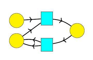
A Petri net can be drawn as a bipartite directed graph with vertices of two kinds: places, drawn as circles, and transitions drawn as squares:

When we run a Petri net, we start by placing a finite number of dots called tokens in each place:

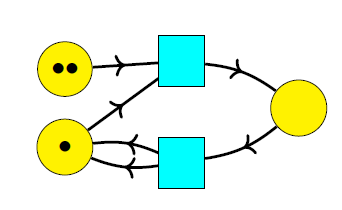
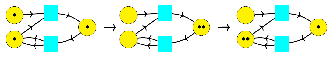
This is called a marking. Then we repeatedly change the marking using the transitions. For example, the above marking can change to this:

and then this:

Thus, the places represent different types of entity, and the transitions are ways that one collection of entities of specified types can turn into another such collection.

Network models serve a different function than Petri nets: they are a general tool for working with networks of many kinds. Mathematically a network model is a lax symmetric monoidal functor where is the free strict symmetric monoidal category on a set Elements of represent different kinds of ‘agents’. Unlike in a Petri net, we do not usually consider processes where these agents turn into other agents. Instead, we wish to study everything that can be done with a fixed collection of agents. Any object is of the form for some thus, it describes a collection of agents of various kinds. The functor maps this object to a category that describes everything that can be done with this collection of agents.

In many examples considered so far, is a category whose morphisms are graphs of some sort whose nodes are agents of types Composing these morphisms corresponds to ‘overlaying’ graphs. Network models of this sort let us design networks where the nodes are agents and the edges are communication channels or shared commitments. In our first paper the operation of overlaying graphs was always commutative:

• John Baez, John Foley, Joe Moeller and Blake Pollard, Network models.

Subsequently Joe introduced a more general noncommutative overlay operation:

• Joe Moeller, Noncommutative network models.

This lets us design networks where each agent has a limit on how many communication channels or commitments it can handle; the noncommutativity lets us take a ‘first come, first served’ approach to resolving conflicting commitments.

Here we take a different tack: we instead take to be a category whose morphisms are processes that the given collection of agents, can carry out. Composition of morphisms corresponds to carrying out first one process and then another.

This idea meshes well with Petri net theory, because any Petri net determines a symmetric monoidal category whose morphisms are processes that can be carried out using this Petri net. More precisely, the objects in are markings of and the morphisms are sequences of ways to change these markings using transitions, e.g.:

Given a Petri net, then, how do we construct a network model and in particular, what is the set ? In a network model the elements of represent different kinds of agents. In the simplest scenario, these agents persist in time. Thus, it is natural to take to be some set of ‘catalysts’. In chemistry, a reaction may require a catalyst to proceed, but it neither increases nor decrease the amount of this catalyst present. In everyday life, a door serves as a catalyst: it lets you walk though a wall, and it doesn’t get used up in the process!

For a Petri net, ‘catalysts’ are species that are neither increased nor decreased in number by any transition. For example, in the following Petri net, species is a catalyst:

but neither nor is a catalyst. The transition requires one token of type as input to proceed, but it also outputs one token of this type, so the total number of such tokens is unchanged. Similarly, the transition requires no tokens of type as input to proceed, and it also outputs no tokens of this type, so the total number of such tokens is unchanged.

In Theorem 11 of our paper, we prove that given any Petri net and any subset of the catalysts of there is a network model

An object says how many tokens of each catalyst are present; is then the subcategory of where the objects are markings that have this specified amount of each catalyst, and morphisms are processes going between these.

From the functor we can construct a category by ‘gluing together’ all the categories using the Grothendieck construction. Because is symmetric monoidal we can use an enhanced version of this construction to make into a symmetric monoidal category. We already did this in our first paper on network models, but by now the math has been better worked out here:

• Joe Moeller and Christina Vasilakopoulou, Monoidal Grothendieck construction.

The tensor product in describes doing processes ‘in parallel’. The category is similar to but it is better suited to applications where agents each have their own ‘individuality’, because is actually a commutative monoidal category, where permuting agents has no effect at all, while is not so degenerate. In Theorem 12 of our paper we make this precise by more concretely describing as a symmetric monoidal category, and clarifying its relation to

There are no morphisms between an object of and an object of when since no transitions can change the amount of catalysts present. The category is thus a ‘disjoint union’, or more technically a coproduct, of subcategories where an element of free commutative monoid on specifies the amount of each catalyst present.

The tensor product on has the property that tensoring an object in with one in gives an object in and similarly for morphisms. However, in Theorem 14 we show that each subcategory also has its own tensor product, which describes doing one process after another while reusing catalysts.

This tensor product is a very cool thing. On the one hand it’s quite obvious: for example, if two people want to walk through a door, they can both do it, one at a time, because the door doesn’t get used up when someone walks through it. On the other hand, it’s mathematically interesting: it turns out to give, not a monoidal category, but something called a ‘premonoidal’ category. This concept, which we explain in our paper, was invented by John Power and Edmund Robinson for use in theoretical computer science.

The paper has lots of pictures involving jeeps and boats, which serve as catalysts to carry people first from a base to the shore and then from the shore to an island. I think these make it clear that the underlying ideas are quite commonsensical. But they need to be formalized to program them into a computer—and it’s nice that doing this brings in some classic themes in category theory!

---

The whole series of posts:

• Part 1. CASCADE: the Complex Adaptive System Composition and Design Environment.

• Part 2. Metron’s software for system design.

• Part 3. Operads: the basic idea.

• Part 4. Network operads: an easy example.

• Part 5. Algebras of network operads: some easy examples.

• Part 6. Network models.

• Part 7. Step-by-step compositional design and tasking using commitment networks.

• Part 8. Compositional tasking using category-valued network models.

• Part 9 – Network models from Petri nets with catalysts.

• Part 10 – Two papers reviewing the whole project.