An interesting situation has arisen. Some people working on applied category theory have been seeking a ‘killer app’: that is, an application of category theory to practical tasks that would be so compelling it would force the world to admit categories are useful. Meanwhile, the UMAP algorithm, based to some extent on category theory, has become very important in genomics:
• Leland McInnes, John Healy and James Melville, UMAP: uniform manifold approximation and projection for dimension reduction.
But while practitioners have embraced the algorithm, they’re still puzzled by its category-theoretic underpinnings, which are discussed in Section 2 of the paper. (You can read the remaining sections, which describe the algorithm quite concretely, without understanding Section 2.)
I first heard of this situation on Twitter when James Nichols wrote:
Wow! My first sighting of applied category theory: the UMAP algorithm. I’m a category novice, but the resulting adjacency-graph algorithm is v simple, so surely the theory boils down to reasonably simple arguments in topology/Riemannian geometry?
Do any of you prolific ACT tweeters know much about UMAP? I understand the gist of the linked paper, but not say why we need category theory to define this “fuzzy topology” concept, as opposed to some other analytic defn.
Junhyong Kim added:
What was gained by CT for UMAP? (honest question, not trying to be snarky)
Leland McInnes, one of the inventors of UMAP, responded:
It is my math background, how I think about the problem, and how the algorithm was derived. It wasn’t something that was added, but rather something that was always there—for me at least. In that sense what was gained was the algorithm.
I don’t really understand UMAP; for a good introduction to it see the original paper above and also this:
• Nikolay Oskolkov, How Exactly UMAP Works—and Why Exactly It Is Better Than tSNE, 3 October 2019.
tSNE is an older algorithm for taking clouds of data points in high dimensions and mapping them down to fewer dimensions so we can understand what’s going on. From the viewpoint of those working on genomics, the main good thing about UMAP is that it solves a bunch of problems that plagued tSNE. Oskolkov explains what these problems are and how UMAP deals with them. But he also alludes to the funny disconnect between these practicalities and the underlying theory:
My first impression when I heard about UMAP was that this was a completely novel and interesting dimension reduction technique which is based on solid mathematical principles and hence very different from tSNE which is a pure Machine Learning semi-empirical algorithm. My colleagues from Biology told me that the original UMAP paper was “too mathematical”, and looking at the Section 2 of the paper I was very happy to see strict and accurate mathematics finally coming to Life and Data Science. However, reading the UMAP docs and watching Leland McInnes talk at SciPy 2018, I got puzzled and felt like UMAP was another neighbor graph technique which is so similar to tSNE that I was struggling to understand how exactly UMAP is different from tSNE.
He then goes on and attempts to explain exactly why UMAP does so much better than tSNE. None of his explanation mentions category theory.
Since I don’t really understand UMAP or why it does better than tSNE, I can’t add anything to this discussion. In particular, I can’t say how much the category theory really helps. All I can do is explain a bit of the category theory. I’ll do that now, very briefly, just as a way to get a conversation going. I will try to avoid category-theoretic jargon as much as possible—not because I don’t like it or consider it unimportant, but because that jargon is precisely what’s stopping certain people from understanding Section 2.
I think it all starts with this paper by Spivak, which McInnes, Healy and Melville cite but for some reason don’t provide a link to:
• David Spivak, Metric realization of fuzzy simplicial sets.
Spivak showed how to turn a ‘fuzzy simplicial set’ into an ‘uber-metric space’ and vice versa. What are these things?
An ‘uber-metric space’ is very simple. It’s a slight generalization of a metric space that relaxes the usual definition in just two ways: it lets distances be infinite, and it lets distinct points have distance zero from each other. This sort of generalization can be very useful. I could talk about it a lot, but I won’t.
A fuzzy simplicial set is a generalization of a simplicial set.
A simplicial set starts out as a set of vertices (or 0-simplices), a set of edges (or 1-simplices), a set of triangles (or 2-simplices), a set of tetrahedra (or 3-simplices), and so on: in short, a set of n-simplices for each n. But there’s more to it. Most importantly, each n-simplex has a bunch of faces, which are lower-dimensional simplices.
I won’t give the whole definition. To a first approximation you can visualize a simplicial set as being like this:
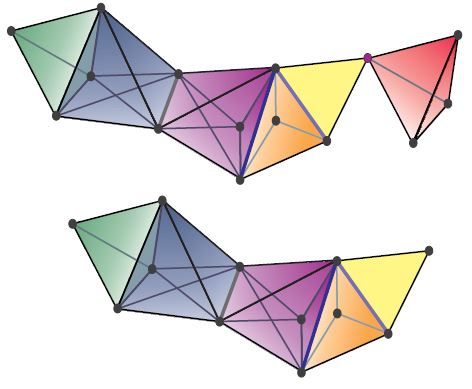
But of course it doesn’t have to stop at dimension 3—and more subtly, you can have things like two different triangles that have exactly the same edges.
In a ‘fuzzy’ simplicial set, instead of a set of n-simplices for each n, we have a fuzzy set of them. But what’s a fuzzy set?
Fuzzy set theory is good for studying collections where membership is somewhat vaguely defined. Like a set, a fuzzy set has elements, but each element has a ‘degree of membership’ that is a number 0 < x ≤ 1. (If its degree of membership were zero, it wouldn't be an element!)
A map f: X → Y between fuzzy sets is an ordinary function, but obeying this condition: it can only send an element x ∈ X to an element f(x) ∈ Y whose degree of membership is greater than or equal to that of x. In other words, we don't want functions that send things to things with a lower degree of membership.
Why? Well, if I'm quite sure something is a dog, and every dog has a nose, then I'm must be at least equally sure that this dog has a nose! (If you disagree with this, then you can make up some other concept of fuzzy set. There are a number of such concepts, and I'm just describing one.)
So, a fuzzy simplicial set will have a set of n-simplices for each n, with each n-simplex having a degree of membership… but the degree of membership of its faces can't be less than its own degree of membership.
This is not the precise definition of fuzzy simplicial set, because I'm leaving out some distracting nuances. But you can get the precise definition by taking a nuts-and-bolts definition of simplicial set, like Definition 3.2 here:
• Greg Friedman, An elementary illustrated introduction to simplicial sets.
and replacing all the sets by fuzzy sets, and all the maps by maps between fuzzy sets.
If you like visualizing things, you can visualize a fuzzy simplicial set as an ordinary simplicial set, as in the picture above, but where an n-simplex is shaded darker if its degree of membership is higher. An n-simplex can’t be shaded darker than any of its faces.
How can you turn a fuzzy simplicial set into an uber-metric space? And how can you turn an uber-metric space into a fuzzy simplicial set?
Spivak focuses on the first question, because the answer is simpler, and it determines the answer to the second using some category theory. (Psst: adjoint functors!)
The answer to the first question goes like this. Say you have a fuzzy simplicial set. For each n-simplex whose degree of membership equals 

This is really just an ordinary metric space: an n-simplex that’s a subspace of Euclidean (n+1)-dimensional space with its usual Euclidean distance function. Then you glue together all these uber-metric spaces, one for each simplex in your fuzzy simplical set, to get a big fat uber-metric space.
This process is called ‘realization’. The key here is that if an n-simplex has a high degree of membership, it gets ‘realized’ as a metric space shaped like a small n-simplex. I believe the basic intuition is that an n-simplex with a high degree of membership describes an (n+1)-tuple of things—its vertices—that are close to each other.
In theory, I should try to describe the reverse process that turns an uber-metric space into a fuzzy simplicial set. If I did, I believe we would see that whenever an (n+1)-tuple of things—that is, points of our uber-metric space—are close, they give an n-simplex with a high degree of membership.
If so, then both uber-metric spaces and fuzzy simplicial sets are just ways of talking about which collections of data points are close, and we can translate back and forth between these descriptions.
But I’d need to think about this a bit more to do a good job of going further, and reading the UMAP paper a bit more I’m beginning to suspect that’s not the main thing that practitioners need to understand. I’m beginning to think the most useful thing is to get a feeling for fuzzy simplicial sets! I hope I’ve helped a bit in that direction. They are very simple things. They are also closely connected to an idea from topological data analysis:
• Nina Otter, Magnitude meets persistence. Homology theories for filtered simplicial sets.
I should admit that McInnes, Healy and Melville tweak Spivak’s formalism a bit. They call Spivak’s uber-metric spaces ‘extended-pseudo-metric spaces’, but they focus on a special kind, which they call ‘finite’. Unfortunately, I can’t find where they define this term. They also only consider a special sort of fuzzy simplicial set, which they call ‘bounded’, but I can’t find the definition of this term either! Without knowing these definitions, I can’t comment on how these tweaks change things.


I’m fairly sure that “finite” just means that the underlying set is finite, which is a standard assumption in data analysis. And “bounded” probably means that there exists an such that
  for all points
  and
and  .
.
Thanks! That definition of “finite” extended extended-pseudo-metric spaces sounds plausible. (I guessed that they were ruling out points whose distance is infinite, but I also knew that couldn’t work, since the resulting category wouldn’t have coproducts.)
I’m still in the dark about what a “bounded” fuzzy simplicial set is: your definition of “bounded” seems more applicable to metric spaces. One huge clue is that they’re wanting an adjunction between “finite” extended-pseudo-metric spaces and “bounded” fuzzy simplicial sets. Another clue is they call the category of “bounded” fuzzy simplicial sets Fin-sFuzz. Both these clues point to “bounded” being some sort of finiteness condition.
(Obviously—though not from anything I said here, since I was hiding the concept of ‘degeneracies’—a fuzzy simplicial set can’t have a finite total number of n-simplices for all n.)
I think another clue is that the metric space they send a fuzzy n-simplex to isn’t to the solid n-simplex Spivak uses, but just its set of n+1 corners. That seems consistent with the idea that a “finite” extended pseudo-metric space is supposed to have a finite underlying set of points. But the realization functor is extended to general fuzzy simplicial set via colimits, so in order to keep the underlying set of the result finite, it seems like we’d have to restrict to only those fuzzy simplicial sets that can be expressed as the colimits of a finite collection of individual fuzzy simplices.
Surely you also need here, to make this shape a simplex instead of a hyperplane.
It’s also interesting that a fuzzy simplex with membership degenerates to a point. (Presumably it isn’t really a point but rather a whole simplex’s worth of points whose distances from one another are all zero, showing why this must be allowed.)
Right, I need those to be nonnegative. I’ll fix that.
Recently, I made some slides explaining the mathematics and implementational details of the UMAP algorithm as it was at the end of summer 2019. The target audience was mathematically-oriented machine learning researchers. Honestly, they didn’t work very well as presentation slides as there is too much information in there, but some might find them useful as a summary and guide to some of the themes. Here they are on SlideShare: https://www.slideshare.net/UmbertoLupo/umap-mathematics-and-implementational-details
This explanation “UMAP Uniform Manifold Approximation and Projection for Dimension Reduction | SciPy 2018 |” https://www.youtube.com/watch?v=nq6iPZVUxZU on YouTube was done by McInnes to describe his python implementation of UMAP. It doesn’t really use category theory but it does have a typical diagram of local mappings from overlapping open sets on a manifold to subsets of R^n and an explanation of how the metrical part of the theory is important.
McInnes also has a couple of theorems from category theory on slides as he moves along, although he doesn’t really go deeply into their content, rather he says they allow him to apply some efficient measurements and statistical (fuzzy) operations.
Thanks John for this exposition. With my very naive understanding of CT, I am still wondering why the construction invoked CT as opposed to just geometrical/topological concepts.
On a different note, several years ago during a sabbatical at Oxford Math Inst with Minhyong (https://www.maths.ox.ac.uk/people/minhyong.kim), we were thinking about data analysis application of simplicial sets–however, I could think of actual data that implies an n-simplex, other than triangulation by 1-simplex. And, I believe in the UMAP paper, the authors actually only use 1-simplices.
They use a very strange definition of extended metric space. Spivak uses the sane definition in which distances can be but the triangle inequality works as expected, giving allowing e.g. distances between different connected components to be
  . They however have that distances
 OR
OR  . This seems to me to ruin all nice properties of the metric, in particular its interpretation as a functor to the totally ordered set
 ![[0,\infty]](https://s0.wp.com/latex.php?latex=%5B0%2C%5Cinfty%5D&bg=ffffff&fg=333333&s=0&c=20201002) .
.
don’t count in the triangle inequality: i.e.
First I thought this was just a clumsy writeup thinko, but they seem to genuinely use this in their also somewhat strange definition of local metric which is defined as
:
if or
or  and
and  otherwise (I guess they should add by hand that
  if
if  )
) .
.
and M is the distance on the embedding manifold or an estimate thereof. This satisfies the triangle inequality only with the strange triangle inequality that cheats for
My guess is, this slipped in when they tried to write down what they actually implemented on a computer.
Yes, I noticed that. My impression is that they use ‘infinity’ to mean infinity when doing the category theory, but it means ‘unknown’ or ‘unreliable’ in the algorithm.
The results of Lemma 1 only provide accurate approximations of geodesic distance local to X_i for distances measured from X_i – the geodesic distances between other pairs of points within the neighborhood of X i are not well defined. In deference to this lack of information we defne distances between X_j and X_k in the extended-pseudo metric space local to X_i (where i != j and i != k) to be infnite (local neighborhoods of X_j and X_k will provide suitable approximations).
Subtracting the minimum distance seems to break the triangle equality. E.g., suppose there are three points making a triangle with sides 5,3,3. They all get the same scale, and all other points are far away. You then get a 2,0,0 triangle (multiplied by some scale).
The second para was meant to be quoted.
You have some knowledge about the distance: that they have to satisfy the triangle inequality, so one would expect “the French railway metric” i.e. for
for  ,
,  .
.
(this is called the French railway metric because basically all railroads in France lead to Paris).
(I think I failed to comment properly before..)
Thank you John for writing this so fast. I guess, being naive, I still am unclear with respect to the category theory part versus standard geometry part.
On a different note, Minhyong (http://people.maths.ox.ac.uk/kimm/) and I used to discuss data analysis applications of simplicial structures and I really couldn’t think of real data that has information on n-simplex for n>2. I think all of the topological data analysis out there “create” n-simplices from pair-wise measurements by triangulation. If that is the case, is there real foundation for that kind of approach?
Thanks….
Junhyong wrote:
A specific question might help, since I can’t tell what you’re unclear about.
A balloon has a hole in it, which in ordinary topology cannot be detected by its first homology group, only its 2nd homology group (a higher-dimensional thing). But we can represent a balloon by a cloud of points in 3d space, and all we need to keep track of is the distances between pairs of points. Persistent homology can then tell that the balloon has a hole in it.
By the way, if we have a bunch of emails, we can build up a simplicial set where an n-simplex is an email that was sent to n+1 people, who are the vertices of that email. So it’s easy to find data structures that are best described using higher-dimensional simplicial sets.
Thanks for writing this up! It seems that most of this algebraic geometry is needed to motivate working with a weighted k-nearest-neighbours (kNN) graph of the dataset (where by “weighted” I mean that the edges have weights, with shorter edges having larger weights). Do you think it’s fair to say that? Because certainly many algorithms before UMAP, including t-SNE, were based on a weighted kNN graph; and it isn’t very clear to me if the categorical treatment in the UMAP paper is just providing a mathematical rationale to that classical computer science approach, or is going beyond.
One aspect where UMAP is different from t-SNE is its loss function. So what I would be very interested to understand, is how much the cross-entropy loss function that UMAP uses follows from all the fuzzy simplicial set theory. Is it something that falls out naturally from the theory? If yes, this I think would be an important contribution. The paper (section 2.3) does not make it very clear to me. What is your perspective here?
By the way, I don’t think Nikolay Oskolkov’s argument for why UMAP is “better” than tSNE is correct. I wrote about it here: https://twitter.com/hippopedoid/status/1227731600647081984
Maybe someone who really understands the UMAP algorithm can answer your questions. So far my feeling is that the category theory and simplicial set theory in this paper are largely separate from the actual algorithm. They are simple, beautiful, and potentially useful in this sort of problem (since they’re already widely used in topological data analysis). But I don’t see much of their power showing up in the algorithm. I might be missing the point.
(By the way, there’s no algebraic geometry at all in this paper. Algebraic geometry means something rather specific, not just any combination of algebraic and geometric ideas.)
The slides I posted above should answer your questions, but please let me know if not and I’ll be happy to clarify! (Not affiliated to the authors particularly, just a fan of the intersection between category theory/algebraic topology, high-performance computing, and machine learning :-).)
Thanks for the pointer! I looked through your slides, but am still not sure what exactly are your answer to my questions. Would very much appreciate if you could answer them directly. I think it boils down to only one question: does this mathematics provide a rationale for the general setting (“embedding kNN graph of the data via some kind of force-directed layout algorithm is a good idea”), or does it uniquely motivate this specific loss function?
Sure, no problem!
I think it is fair to say that. Though I’d refine the statement to say that the category theory and computational topology are used as a justification for the specific form of the final weighted graph. Schematically:
a) consider ways to compute a meaningful topological signature from a finite “metric-like” space;
b) Spivak’s framework (appropriately modified) says that the “right thing” to look at, categorically speaking, is a “fuzzy singular homology” functor which sends a “metric-like” space to a “fuzzy simplicial set”;
c) due to combinatorial explosions, it is only reasonable to ask a computer to store a part of the resulting fuzzy simplicial set, namely the fuzzy set of its edges (1-simplices);
d) a quick computation shows that the resulting structure is that of a weighted graph with exponential weights (due to logarithms appearing in Spivak’s theory);
e) the fuzzy set framework lends itself to local-to-global procedures via fuzzy unions — this is an extra bonus;
f) the fuzzy set cross-entropy is quite a natural way of measuring dissimilarity between fuzzy sets (you essentially regard a fuzzy set as a “field” of Bernoulli random variables). So this type of loss seems well-adapted to the algorithm’s theoretical guiding principles.
I hope this helps!
It seems I cannot reply to your last comment (perhaps because it’s too nested), so I’m replying here instead.
Thanks! This is very helpful. The points in your list that are most interesting for me are (d) and (f). Regarding (d), I did not realize that the exponentially decaying weights is something that follows naturally from Spivak’s theory! I have now re-read Section 3.1 of the UMAP preprint, and it does not make mention this at all. If true, this is interesting. However, practically speaking, Gaussian kernel (which is exponentially decaying) is by far the most often used kernel in machine learning and statistics, so while it’s nice to have an additional motivation, it does not really yield anything new.
Point (f) is the most interesting one. The cross-entropy loss is arguably the most important UMAP’s ingredient for the comparison with t-SNE. (By the way, this loss was introduced in a method called largeVis back in 2016 without any category theory, and I largely see UMAP as providing a motivation for largeVis). So I think it’s important to understand if there could be various reasonable ways to measure fuzzy set dissimilarity or whether cross-entropy is unique and/or somehow preferred.
Spivak’s paper is at
Click to access metric_realization.pdf
I don’t know category theory, so I may have missed something big, but it doesn’t seem to me that logarithms play an important role. I think (1-x)/x, for example, would work just as well as -lg(x).
Also, the Gaussian uses squared distance, not distance, and squared distance is not a metric.
@Graham, you’re right to say that about logarithms. Indeed I raised that point to one of the authors of UMAP a few weeks ago, and he agreed that the theory should carry through with more general functions (monotonically increasing from $-\infty$ to $+\infty$, roughly speaking). Apparently, the logarithm also happens to give good results in practice, so UMAP sticks to this original choice.
Indeed, the kernel is not really Gaussian in UMAP, it’s rather a “Laplace kernel”.
The appearance of the logarithm does not follow from Spivak’s theory: he just chooses that function out of the blue, and any function with a few nice properties would work as well for his results.
John: Spivak introduces the logarithm in the second paragraph of Section 3 in http://math.mit.edu/~dspivak/files/metric_realization.pdf, though we all agree that that choice is not crucial for the theory.
What I had meant is that the UMAP authors make minimal adaptations of this framework to the case of finite metric spaces, including the non-unique choice of using the logarithm! In UMAP, the finite extended pseudo-metric spaces in Definition 7 are the counterparts of Spivak’s
  and the logarithm seems to me to have been inspired by Spivak’s — though I’d agree that there is no well-defined rigorous link.
One could maybe interpret the points in
  as the vertices of Spivak’s geometric realizations of the standard fuzzy
  -simplices, in the sense that in both cases pairwise distances grow linearly with
  .
.
This paper by Ting, Huang, and Jordan, https://arxiv.org/abs/1101.5435, I think gives a good framework for graph kernels including kNN graphs and approximating embeddings. Also, the classic papers by Coifman on diffusion maps (e.g., https://www.pnas.org/content/102/21/7426). I think these are more straightforward standard manifold learning treatments.
(I am still trying to understand enough to ask John a more intelligent question on the CT framework of the UMAP and how it motivates the algorithm part.)
I’m a biologist who uses UMAP in my work. I have a math background and just spent a year learning category and topos theory, primarily to understand the UMAP paper. I don’t regret this, because category theory is fun. But the main lesson was:
The details of UMAP are not constrained by category theory.
Instead, the algorithm’s details seem to have been chosen to make it work in practice, and sometimes justified by analogy to concepts from pure math. For example
UMAP’s score function is based on probability theory, but probability appears nowhere in the Barr/Spivak framework.
Spivak’s use of the log function was arbitrary, but it plays a key role in UMAP (as mentioned above).
UMAP sets the distance between nearest-neighboring data points to zero. This is justified by local connectivity of the embedding manifold. But manifolds are always locally connected – this instead makes it non-Hausdorff (and not actually a manifold).
It might be possible to come up with a categorical framework from which you can derive UMAP’s details, and that would be a great topic of research which could lead to further improvements in the algorithm. For example, this would involve modifying the Barr/Spivak framework so that UMAP’s cross-entropy score emerges naturally.
UMAP is a great algorithm, whose inventors were inspired by pure math. Which is fine: the discovery of benzene’s ring structure was inspired by a dream of a snake eating its own tail. Whatever works.
But to claim right now that UMAP is a killer app for category theory would be a mistake. This will just lead to disappointment for those who actually work through the details, and won’t help the field of applied category theory gain respect.
I have not learned category theory. I suppose I’m waiting for that killer app that will make me take it seriously. Non-linear dimensionality reduction (NLDR) would never be that that application for me because the problem it attempts to solve is so vaguely defined. There is no best way of mapping points on the Earth’s surface to 2D, and the data sets that are fed into NLDR algorithms are much harder than that. Wikipedia lists 29 NLDR algorithms ( https://en.wikipedia.org/wiki/Nonlinear_dimensionality_reduction ) and I think each one has it’s own unique selling point. UMAP is not the only one where the mathematical inspiration behind the algorithm is more interesting than the algorithm itself.
I get the impression that much of the popularity of t-SNE and UMAP is their ability to detect clusters. But then, I think: if you want to detect clusters, wouldn’t it be better to use a clustering algorithm which is designed for that purpose and not constrained by the need to make nice pictures?
I think I have some insight into why UMAP works well, but it has nothing to do with category theory.
In a high dimensional space, all the distances between pairs of points from a finite set are about the same. This isn’t quite true of course, but if someone hands you a set of high dimensional real-world data, it’s a good guess. Taking the MNIST data for example, over 99% of the pairwise distances are between 9 and 14. Almost all are between 5 and 15. If these are to be sensibly mapped to 2 dimensions, something major needs to happen to this distribution of distances.
Puzzle: how many points can you place in the plane so that the maximum distance between any pair is no more than 3 times the minimum?
To make local distances from each point, UMAP subtracts the distance to the nearest neighbour. This is done to ensure local connectedness. But it has a big effect on the distribution of distances. I guess that roughly speaking, the range 9 to 14 becomes 0 to 5 for a typical point in the MNIST data.
UMAP then converts these to asymmetric similarities which have to be made symmetric using some function f(p,q). I would expect this to satisfy f(p,p) = p. If a pair of similarities are already the same, why would you change them? In UMAP f(p,p) = 2p – p^2. So, for example, a similarity of .9 becomes .99. This corresponds to more squashing of small distances.
In summary, the way that UMAP ensures local connectivity and symmetry have drastic side effects on distances, and these side effects are a good thing if you are making a large reduction in dimensionality.
It seems from a TDA-theoretic point of view that all 0-simplex as data points should just have degree of membership 1 by default. Is this correct? At least in an UMAP example it shows like that.