Fisher’s Fundamental Theorem (Part 2)

Here’s how Fisher stated his fundamental theorem:

The rate of increase of fitness of any species is equal to the genetic variance in fitness.

But clearly this is only going to be true under some conditions!

A lot of early criticism of Fisher’s fundamental theorem centered on the fact that the fitness of a species can vary due to changing external conditions. For example: suppose the Sun goes supernova. The fitness of all organisms on Earth will suddenly drop. So the conclusions of Fisher’s theorem can’t hold under these circumstances.

I find this obvious and thus uninteresting. So, let’s tackle situations where the fitness changes due to changing external conditions later. But first let’s see what happens if the fitness isn’t changing for these external reasons.

What’s ‘fitness’, anyway? To define this we need a mathematical model of how populations change with time. We’ll start with a very simple, very general model. While it’s often used in population biology, it will have very little to do with biology per se. Indeed, the reason I’m digging into Fisher’s fundamental theorem is that it has a mathematical aspect that doesn’t require much knowledge of biology to understand. Applying it to biology introduces lots of complications and caveats, but that won’t be my main focus here. I’m looking for the simple abstract core.

The Lotka–Volterra equation

The Lotka–Volterra equation is a simplified model of how populations change with time. Suppose we have $n$ different types of self-replicating entity. We will call these entities replicators. We will call the types of replicators species, but they do not need to be species in the biological sense!

For example, the replicators could be organisms of one single biological species, and the types could be different genotypes. Or the replicators could be genes, and the types could be alleles. Or the replicators could be restaurants, and the types could be restaurant chains. In what follows these details won’t matter: we’ll have just have different ‘species’ of ‘replicators’.

Let $P_i(t)$ or just $P_i$ for short, be the population of the $i$ th species at time $t.$ We will treat this population as a differentiable real-valued function of time, which is a reasonable approximation when the population is fairly large.

Let’s assume the population obeys the Lotka–Volterra equation:

$\displaystyle{ \frac{d P_i}{d t} = f_i(P_1, \dots, P_n) \, P_i }$

where each function $f_i$ depends in a differentiable way on all the populations. Thus each population $P_i$ changes at a rate proportional to $P_i,$ but the ‘constant of proportionality’ need not be constant: it depends on the populations of all the species.

We call $f_i$ the fitness function of the $i$ th species. Note: we are assuming this function does not depend on time.

To write the Lotka–Volterra equation more concisely, we can create a vector whose components are all the populations:

$P = (P_1, \dots , P_n).$

Let’s call this the population vector. In terms of the population vector, the Lotka–Volterra equation become

$\displaystyle{ \dot P_i = f_i(P) P_i}$

where the dot stands for a time derivative.

To define concepts like ‘mean fitness’ or ‘variance in fitness’ we need to introduce probability theory, and the replicator equation.

The replicator equation

Starting from the populations $P_i$ , we can work out the probability $p_i$ that a randomly chosen replicator belongs to the $i$ th species. More precisely, this is the fraction of replicators belonging to that species:

$\displaystyle{ p_i = \frac{P_i}{\sum_j P_j} }$

As a mnemonic, remember that the big Population $P_i$ is being normalized to give a little probability $p_i.$ I once had someone scold me for two minutes during a talk I was giving on this subject, for using lower-case and upper-case P’s to mean different things. But it’s my blog and I’ll do what I want to.

How do these probabilities $p_i$ change with time? We can figure this out using the Lotka–Volterra equation. We pull out the trusty quotient rule and calculate:

$\displaystyle{ \dot{p}_i = \frac{\dot{P}_i \left(\sum_j P_j\right) - P_i \left(\sum_j \dot{P}_j \right)}{\left( \sum_j P_j \right)^2 } }$

Then the Lotka–Volterra equation gives

$\displaystyle{ \dot{p}_i = \frac{ f_i(P) P_i \; \left(\sum_j P_j\right) - P_i \left(\sum_j f_j(P) P_j \right)} {\left( \sum_j P_j \right)^2 } }$

Using the definition of $p_i$ this simplifies and we get

$\displaystyle{ \dot{p}_i = f_i(P) p_i - \left( \sum_j f_j(P) p_j \right) p_i }$

The expression in parentheses here has a nice meaning: it is the mean fitness. In other words, it is the average, or expected, fitness of a replicator chosen at random from the whole population. Let us write it thus:

$\displaystyle{ \overline f(P) = \sum_j f_j(P) p_j }$

This gives the replicator equation in its classic form:

$\displaystyle{ \dot{p}_i = \left( f_i(P) - \overline f(P) \right) \, p_i }$

where the dot stands for a time derivative. Thus, for the fraction of replicators of the $i$ th species to increase, their fitness must exceed the mean fitness.

The moral is clear:

To become numerous you have to be fit.
To become predominant you have to be fitter than average.

This picture by David Wakeham illustrates the idea:

The fundamental theorem

What does the fundamental theorem of natural selection say, in this context? It says the rate of increase in mean fitness is equal to the variance of the fitness. As an equation, it says this:

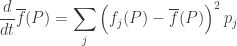
$\displaystyle{ \frac{d}{d t} \overline f(P) = \sum_j \Big( f_j(P) - \overline f(P) \Big)^2 \, p_j }$

The left hand side is the rate of increase in mean fitness—or decrease, if it’s negative. The right hand side is the variance of the fitness: the thing whose square root is the standard deviation. This can never be negative!

A little calculation suggests that there’s no way in the world that this equation can be true without extra assumptions!

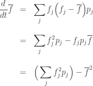
We can start computing the left hand side:

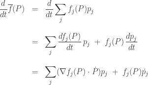
$\begin{array}{ccl} \displaystyle{\frac{d}{d t} \overline f(P)} &=& \displaystyle{ \frac{d}{d t} \sum_j f_j(P) p_j } \\ \\ &=& \displaystyle{ \sum_j \frac{d f_j(P)}{d t} \, p_j \; + \; f_j(P) \, \frac{d p_j}{d t} } \\ \\ &=& \displaystyle{ \sum_j (\nabla f_j(P) \cdot \dot{P}) p_j \; + \; f_j(P) \dot{p}_j } \end{array}$

Before your eyes glaze over, let’s look at the two terms and think about what they mean. The first term says: the mean fitness will change since the fitnesses $f_j(P)$ depend on $P,$ which is changing. The second term says: the mean fitness will change since the fraction $p_j$ of replicators that are in the $j$ th species is changing.

We could continue the computation by using the Lotka–Volterra equation for $\dot{P}$ and the replicator equation for $\dot{p}.$ But it already looks like we’re doomed without invoking an extra assumption. The left hand side of Fisher’s fundamental theorem involves the gradients of the fitness functions, $\nabla f_j(P).$ The right hand side:

$\displaystyle{ \sum_j \Big( f_j(P) - \overline f(P) \Big)^2 \, p_j }$

does not!

This suggests an extra assumption we can make. Let’s assume those gradients $\nabla f_j$ vanish!

In other words, let’s assume that the fitness of each replicator is a constant, independent of the populations:

$f_j(P_1, \dots, P_n) = f_j$

where $f_j$ at right is just a number.

Then we can redo our computation of the rate of change of mean fitness. The gradient term doesn’t appear:

$\begin{array}{ccl} \displaystyle{\frac{d}{d t} \overline f(P)} &=& \displaystyle{ \frac{d}{d t} \sum_j f_j p_j } \\ \\ &=& \displaystyle{ \sum_j f_j \dot{p}_j } \end{array}$

We can use the replicator equation for $\dot{p}_j$ and get

$\begin{array}{ccl} \displaystyle{ \frac{d}{d t} \overline f } &=& \displaystyle{ \sum_j f_j \Big( f_j - \overline f \Big) p_j } \\ \\ &=& \displaystyle{ \sum_j f_j^2 p_j - f_j p_j \overline f } \\ \\ &=& \displaystyle{ \Big(\sum_j f_j^2 p_j\Big) - \overline f^2 } \end{array}$

This is the mean of the squares of the $f_j$ minus the square of their mean. And if you’ve done enough probability theory, you’ll recognize this as the variance! Remember, the variance is

$\begin{array}{ccl} \displaystyle{ \sum_j \Big( f_j - \overline f \Big)^2 \, p_j } &=& \displaystyle{ \sum_j f_j^2 \, p_j - 2 f_j \overline f \, p_j + \overline f^2 p_j } \\ \\ &=& \displaystyle{ \Big(\sum_j f_j^2 \, p_j\Big) - 2 \overline f^2 + \overline f^2 } \\ \\ &=& \displaystyle{ \Big(\sum_j f_j^2 p_j\Big) - \overline f^2 } \end{array}$

Same thing.

So, we’ve gotten a simple version of Fisher’s fundamental theorem. Given all the confusion swirling around this subject, let’s summarize it very clearly.

Theorem. Suppose the functions $P_i \colon \mathbb{R} \to (0,\infty)$ obey the equations

$\displaystyle{ \dot P_i = f_i P_i}$

for some constants $f_i.$ Define probabilities by

$\displaystyle{ p_i = \frac{P_i}{\sum_j P_j} }$

Define the mean fitness by

$\displaystyle{ \overline f = \sum_j f_j p_j }$

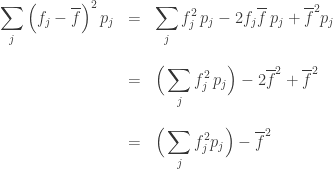
and the variance of the fitness by

$\displaystyle{ \mathrm{Var}(f) = \sum_j \Big( f_j - \overline f \Big)^2 \, p_j }$

Then the time derivative of the mean fitness is the variance of the fitness:

$\displaystyle{ \frac{d}{d t} \overline f = \mathrm{Var}(f) }$

This is nice—but as you can see, our extra assumption that the fitness functions are constants has trivialized the problem. The equations

$\displaystyle{ \dot P_i = f_i P_i}$

are easy to solve: all the populations change exponentially with time. We’re not seeing any of the interesting features of population biology, or even of dynamical systems in general. The theorem is just an observation about a collection of exponential functions growing or shrinking at different rates.

So, we should look for a more interesting theorem in this vicinity! And we will.

Before I bid you adieu, let’s record a result we almost reached, but didn’t yet state. It’s stronger than the one I just stated. In this version we don’t assume the fitness functions are constant, so we keep the term involving their gradient.

Theorem. Suppose the functions $P_i \colon \mathbb{R} \to (0,\infty)$ obey the Lotka–Volterra equations:

$\displaystyle{ \dot P_i = f_i(P) P_i}$

for some differentiable functions $f_i \colon (0,\infty)^n \to \mathbb{R}$ called fitness functions. Define probabilities by

$\displaystyle{ p_i = \frac{P_i}{\sum_j P_j} }$

Define the mean fitness by

$\displaystyle{ \overline f(P) = \sum_j f_j(P) p_j }$

and the variance of the fitness by

$\displaystyle{ \mathrm{Var}(f(P)) = \sum_j \Big( f_j(P) - \overline f(P) \Big)^2 \, p_j }$

Then the time derivative of the mean fitness is the variance plus an extra term involving the gradients of the fitness functions:

$\displaystyle{\frac{d}{d t} \overline f(P)} = \displaystyle{ \mathrm{Var}(f(P)) + \sum_j (\nabla f_j(P) \cdot \dot{P}) p_j }$

The proof just amounts to cobbling together the calculations we have already done, and not assuming the gradient term vanishes.

Acknowledgements

After writing this blog article I looked for a nice picture to grace it. I found one here:

• David Wakeham, Replicators and Fisher’s fundamental theorem, 30 November 2017.

I was mildly chagrined to discover that he said most of what I just said more simply and cleanly… in part because he went straight to the case where the fitness functions are constants. But my mild chagrin was instantly offset by this remark:

Fisher likened the result to the second law of thermodynamics, but there is an amusing amount of disagreement about what Fisher meant and whether he was correct. Rather than look at Fisher’s tortuous proof (or the only slightly less tortuous results of latter-day interpreters) I’m going to look at a simpler setup due to John Baez, and (unlike Baez) use it to derive the original version of Fisher’s theorem.

So, I’m just catching up with Wakeham, but luckily an earlier blog article of mine helped him avoid “Fisher’s tortuous proof” and the “only slightly less tortuous results of latter-day interpreters”. We are making progress here!

(By the way, a quiz show I listen to recently asked about the difference between “tortuous” and “torturous”. They mean very different things, but this particular case either word would apply.)

My earlier blog article, in turn, was inspired by this paper:

• Marc Harper, Information geometry and evolutionary game theory.

The whole series:

• Part 1: the obscurity of Fisher’s original paper.

• Part 2: a precise statement of Fisher’s fundamental theorem of natural selection, and conditions under which it holds.

• Part 3: a modified version of the fundamental theorem of natural selection, which holds much more generally.

• Part 4: my paper on the fundamental theorem of natural selection.

This entry was posted on Tuesday, September 29th, 2020 at 3:03 pm and is filed under biology, mathematics. You can follow any responses to this entry through the RSS 2.0 feed. You can leave a response, or trackback from your own site.

21 Responses to Fisher’s Fundamental Theorem (Part 2)

Hendrik Boom says:

29 September, 2020 at 9:15 pm

Upper-case vs lower-case P’s is an issue when using hand writing. Not so much when type-set, as you do here.
Even when hand-writing, there’s no problem with, say, distinguishing A from a.

Reply
Raphael says:

29 September, 2020 at 9:36 pm

Very interesting, I am curious to see the thing for non-constant f! Crazy question: If one would assume some structural relation between averages values and differentiation (like in the mean value theorem) then the variance would be related to second derivatives and we would have an analog of the heat equation. Is there some way to make sense of this?

Reply
- John Baez says:
  
  29 September, 2020 at 10:18 pm
  
  I just added a version for nonconstant fitness functions that follows from all the calculations I already did. It’s not very charismatic.
  
  I don’t know how to get second derivatives or the Laplacian into the game here.
  
  There are other things to say, which I hope to discuss next time!
  
  Reply
- Marc Harper says:
  
  29 September, 2020 at 11:54 pm
  
  IIRC, if you view the replicator equation geometrically as deriving from the Fisher information metric, it’s possible to use standard methods from Riemannian geometry to compute a heat equation on the same metric. From the information geometry side, see Guy Lebanon’s thesis “Riemannian Geometry and Statistical Machine Learning”.
  
  Reply
  - Raphael says:
    
    30 September, 2020 at 5:31 am
    
    Thank you very much Mark, quite interesting! Now, I try to understand if we can give any sensical interpretation of replicator time evolution in terms of heat diffusion.
    
    Reply
  - John Baez says:
    
    30 September, 2020 at 2:29 pm
    
    I’d say the heat equation is more connected to Brownian motion, which might serve as a way of thinking about a random walk, e.g. due to mutations. Someone should have tried this—I don’t know.
    
    Reply
Marc Harper says:

29 September, 2020 at 11:45 pm

Hi John!

For a less trivial example, FFT (without the extra term) holds for linear symmetric fitness landscapes of the form $f(p) = Ap$ where $A = A^T$ for the matrix $A$ . This goes back at least to [1], to the earlier form of the replicator equation that explicitly described $n$ alleles at a gene locus (which is assumed to be linear and symmetric). More generally, FFT holds for landscapes $f$ that are Euclidean gradients (see Theorem 19.5.1 of [2], or [3]).

There’s a neat little calculation here that illuminates the difference between the replicator equation and the (Fisher / Shahshahani) gradient. If we have a fitness landscape that isn’t a Euclidean gradient we can nevertheless compute the (Shahshahani) gradient of the (IIRC half of the) mean fitness. Starting with $f(p) = Ap$ for arbitrary $A$ , computing the gradient results in a replicator equation with landscape $g(p) = B p$ where $B = (A + A^T) / 2$ is the symmetrization of $A$ .

If we take a landscape for an anti-symmetric matrix like the rock-paper-scissors game, this gradient is zero everywhere, so the dynamic is motionless. In contrast, the phase portrait of the replicator equation for the RSP landscape consists of concentric cycles about a non-attracting equilibrium (with the KL-divergence constant along the cycles instead of being a Lyapunov function.)

In this case the mean fitness is zero, so away from the rest point at (1/3, 1/3, 1/3) FFT wouldn’t work without the extra terms as the variance would be non-zero. The extra term of $<df/dt>$ is the negative of the variance, which can be directly shown by computing all the terms out.

In general (again IIRC, it’s been a while) the gradient is something like $g(p) = (1/2) (f(p) + p^T J(f(p)))$ where $J$ is the Jacobian matrix, which should reduce to the example above for $f(p) = A p$ .

[1] S. Shahshahani, “A New Mathematical Framework for the Study of Linkage and Selection” (1979)
[2] Hofbauer and Sigmund, “Evolutionary Games and Population Dynamics” (1998)
[3] J. Hofbauer, “The selection-mutation equation” (1985)

Reply
- John Baez says:
  
  30 September, 2020 at 1:20 am
  
  I definitely want to talk about less trivial examples. Thanks for helping line them up. I was just reading Evolutionary Games and Population Dynamics. I couldn’t find where they talk about Fisher’s fundamental theorem. Theorem 19.5.1, eh? I’ll check it out.
  
  Reply
  - Marc Harper says:
    
    30 September, 2020 at 2:27 am
    
    It’s stated as equation 19.18 after the proof of Theorem 19.5.1 (which it follows from), but not named as FFT (or cited). Theorem 19.5.1 is part of Theorem 3 in [3]. See also Theorems 1, 2, and 3 in my paper, which are these theorems and the information theory analog of FFT.
    
    Reply
  - John Baez says:
    
    1 October, 2020 at 12:57 am
    
    I’m finding Theorem 19.5.1 a bit frustrating. The statement gives two mutually incompatible equations involving $\dot{x}_i:$
    
    $\dot{x}_i = f_i(\mathbf{x}) = \frac{\partial V}{\partial x_i}$
    
    and
    
    $\dot{x}_i = \hat{f}_i(\mathbf{x}) = x_i (f_i(\mathbf{x}) - \overline{f}(\mathbf{x}))$
    
    My guess is that the first equation for $\dot{x}_i$ is “just for fun”, not something we should use, though we should use
    
    $f_i(\mathbf{x}) = \frac{\partial V}{\partial x_i}$
    
    The second equation for $\dot{x}_i$ is the one actually used in the proof.
    
    Is that right?
    
    Then in (19.18) below, $\dot{\mathbf{x}}$ is the time derivative of a point moving around on the probability simplex, defined to have components
    
    $\dot{x}_i = \hat{f}_i(\mathbf{x}) = x_i (f_i(\mathbf{x}) - \overline{f}(\mathbf{x})$
    
    Right?
    
    Reply
    - Marc Harper says:
      
      1 October, 2020 at 5:46 am
      
      Yes that proof isn’t the most enlightening / well explained — they reuse the dummy variable $x$ in a confusing way as you’ve noted.
      
      FFT can also be shown directly as follows.
      
      Assuming that $f_i = \frac{\partial V}{\partial x_i}$ and that $x$ follows the replicator equation, using the chain rule we have that
      
      $\begin{array}{ccl} \displaystyle{ \frac{dV}{dt}} &=& \displaystyle{ \sum_i{ \frac{\partial V}{\partial x_i} \dot{x}_i } } \\ \\ &=& \displaystyle{ \sum{f_i \dot{x}_i} } \\ \\ &=& \displaystyle{ \sum{f_i \left(x_i (f_i - \bar{f}) \right)} } \\ \\ &=& \displaystyle{ \sum{x_i \left(f_i - \bar{f} \right)^2} } \end{array}$
      
      The last step is bit tricky and follows because we can subtract
      
      $\displaystyle{ 0 = \sum{x_i \left(f_i - \bar{f} \right) \bar{f}} }$
      
      That sum is zero because $\bar{f}$ factors out (doesn’t depend on i) and so
      
      $\displaystyle{ \bar{f} \sum_i x_i \left(f_i - \bar{f} \right) = \bar{f} \left((\sum_i x_i f_i) - (\sum_i x_i) \bar{f} \right) }$
      
      and since $\sum_i {x_i} = 1$ and $\bar{f} = \sum_i {x_i f_i},$ we have
      
      $\bar{f} (\bar{f} - \bar{f}) = 0$
      
      So FFT works for the gradient because of the chain rule. In the text Theorem 7.8.1 (on page 82) does this calculation for the special case that $f(x) = Ax$ for a symmetric matrix $A$ .
      
      More generally, if one looks at the mean fitness for an arbitrary $f$ , there’s an extra term $\langle \frac{df}{dt} \rangle$ (like in Wakeham’s article). Why? If we start instead with a vector-valued function $V$ and ask about the time derivative of its mean, we have that
      
      $\dot{x \cdot V} = \dot{x} \cdot{V} + x \cdot \dot{V}$
      
      The right most term can be manipulated into $\dot{x} \cdot ( x \circ \nabla V)$ where $\circ$ denotes the element-wise product (Hadamard product). The two terms are equal when $V = x \circ \nabla V$ and it’s easy to see that happens if $V = A x$ for a symmetric matrix $A$ . That makes the two terms of $\dot{x \cdot V}$ equal so we get twice the variance (e.g. the extra term in FFT is just another copy of the variance). Alternatively, we can start with $V$ as the half-mean fitness so that the time derivative is just the variance.
    - John Baez says:
      
      1 October, 2020 at 7:38 pm
      
      Thanks for your detailed reply—this is really helpful! I’ll try to explain some of this stuff in a nice way.
      
      I fixed the typos, and I’m happy to do so because it gives me a chance to work through the equations in detail.
      
      One thing I can’t fix is this:
      
      Expert blog-commenters know to click “Reply”, not on the comment they’re replying to, but on the comment it was replying to.
      
      If you do this, you create a comment that’s the same width as the comment you’re replying to. If you don’t do this, the comment thread gets skinnier and skinnier, which is especially unpleasant for comments with equations.
    - John Baez says:
      
      5 October, 2020 at 8:08 pm
      
      I’m still confused, Marc, about whether the $x_i$ in your argument are supposed to be probabilities or populations. That is: are they constrained to sum to 1, or not?
      
      In your calculation you say they sum to 1, so let’s assume that.
      
      If they are constrained to sum to 1, I’m not sure what
      
      $\displaystyle{ \frac{\partial V}{\partial x_i} }$
      
      means, since we can’t change just one $x_i$ while holding the rest fixed. Maybe $V$ is defined on the whole orthant
      
      $\{(x_1, \dots, x_n) : x_i > 0 \}$
      
      so we know what
      
      $\displaystyle{ \frac{\partial V}{\partial x_i} }$
      
      means, but then in your calculation below they sum to 1?
      
      This would solves some problems, but not all, since when we derive the replicator equation from the Lotka–Volterra equation, the right-hand side of the replicator equation actually involves not just the probabilities but actually the populations:
      
      $\dot{p}_i = (f_i(P) - \overline{f}(P)) p_i$
      
      (Here I’m using $p_i$ for probabilities and $P_i$ for populations.) So my next question is, when you write
      
      $\displaystyle{ \frac{\partial V}{\partial x_i} }$
      
      is this partial derivative being evaluated at $p$ (in the simplex) or $P$ (in the orthant)?
    - Marc Harper says:
      
      6 October, 2020 at 4:48 am
      
      For the replicator equation I assumed that the population is infinite and that $\sum_i{p_i} = 1$ . (Above I used $x_i$ from the reference which was intended to match your $p_i$ .) Note if we start from the replicator equation, we have that
      $\sum_i{\dot{p}_i} = 0$
      (even if we don’t assume the proportions sum to 1), so the sum has to be constant and preserved along trajectories (the replicator equation is “forward-invariant”). Anyway in my case only the proportions appear.
      
      As for $\frac{\partial V}{\partial p_i}$ … I think they are just the formal partial derivatives (assuming variable independence) within the context of the multivariate chain rule for $\frac{dV}{dt}$ where all the $p_i$ are implicitly functions of $t$ . IIUC we don’t need to consider the impact of holding some variables constant in this case. If we knew $p_i$ explicitly as functions of $t$ (satisfying constraints), it wouldn’t matter if we used the chain rule as above or rewrote $V$ to a function of $t$ and then took the derivative.
    - John Baez says:
      
      6 October, 2020 at 6:44 pm
      
      Your reply leaves me even more befuddled.
      
      1) In the framework I’m describing in this post the population is never “infinite”. The populations $P_i(t)$ are treated as valued in $(0,\infty).$ This is an idealization which works best for large populations, but using it we get the Lotka–Volterra equations and these equations are the starting-point of my post. These equations make mathematical sense for any positive finite real populations $P_i(t)$ , so we don’t ask question like “what does a population of 2.5 mean?”—we just work with the math. From these equations we derive the replicator equation
      
      $\displaystyle{ \dot{p}_i(t) = f_i(P(t)) p_i(t) - \left( \sum_j f_j(P(t)) p_j(t) \right) p_i(t) }$
      
      for the probabilities $p_i(t)$ . But the replicator equation is not an autonomous system of differential equations for the probabilities, because it involves the populations as well, and many different choices of populations $P_1(t), \dots, P_n(t)$ give the same probabilities
      
      $\displaystyle{ p_i(t) = \frac{P_i(t)}{\sum_j P_j(t)} }$
      
      Thus, the time evolution of the probabilities does not depend on just the probabilities now, but also the choice of populations giving these probabilities. Unless, of course, we make an extra assumption on the nature of the fitness functions $f_i$ , such as that they depend only on the probabilities! This assumption is equivalent to demanding
      
      $f_i(cP_1, \dots, cP_n) = f_i(P_1, \dots, P_n)$
      
      for all $c > 0$ and all $P_1, \dots, P_n > 0.$ This in turn is equivalent to
      
      $\displaystyle{ \sum_j \frac{\partial f_i}{\partial x_j}(x_1, \dots, x_n) = 0 }$
      
      for all $x_1, \dots, x_n > 0.$
      
      2) A partial derivative with respect to one coordinate only makes sense if we know what other coordinate functions are being held constant: the answer depends on that choice. If we have a function $V$ defined on $\mathbb{R}^n$ or the positive orthant,
      
      $\displaystyle{ \frac{\partial V}{\partial x_i} }$
      
      makes sense because implicitly we are holding all the other $n-1$ coordinates $x_1, \dots, x_{i-1}, x_{i+1}, \dots, x_n$ constant. If we have a function $V$ defined only on the simplex, this partial derivative becomes ambiguous, since it’s impossible to change $x_i$ without changing some of the other coordinates. I can imagine ways to disambiguate it, e.g.: take the directional derivative in the direction on the simplex that makes the smallest angle to the vector pointing in the $x_i$ direction in $\mathbb{R}^n.$
      
      Theorem 19.5.1 in Evolutionary Games and Population Dynamics does not address either of these issues, making their proof (and yours) very hard to interpret. I’ve tried a number of ways to get it make sense, and they keep breaking down when I try to write up a proof. Right now I have yet another way in mind, but I’m nervous.
    - Marc Harper says:
      
      7 October, 2020 at 12:30 am
      
      (1) As you point out, we’re talking about two different replicator equations. The reference and I are using an autonomous system of only the population proportions / probabilities that isn’t necessarily derived from a Lotka-Volterra equation.
      
      For a combination of mathematical and conceptual reasons, from my experience with the literature, people tend to use models like
      
      • the replicator equation for “very large” or infinite populations, involving only proportions and with fitness functions that only depend on proportions
      • the Lotka-Volterra for finite yet “continuous” population sizes, so that derivatives or discrete dynamics systems can still be used
      • Markov processes such as the Moran and Wright-Fisher processes for “more realistic” populations (finite with integral population sizes)
      
      (Note I’m not taking issue with your approach and I understand that it retains all the $P_i$ as finite and unbounded.)
      
      (2) Along a trajectory of my replicator equation the population proportions are all functions of a single independent variable, time. Since we’re taking a derivative of a function $V$ along a trajectory of the system with respect to time, there’s no freedom to choose a direction for the derivative, even though $V$ is multivariate when not constrained to the trajectory. So it is a directional derivative with direction determined by the dynamical system. IIUC this applies in the abstract to both our formulations, but your equation has both $P_i$ and $p_i$ (also functions of just time ultimately, and perhaps the directions are often the same up to normalization).
      
      In my case, the derivative of function $V$ (like the mean fitness) along a trajectory can then be understood as
      
      $\displaystyle{ \frac{dV}{dt} = \nabla V \cdot \dot{p} = \sum_i { \frac{\partial V}{\partial p_i} \frac{d p_i}{dt} } }$
      
      where the gradient is given by the partial derivatives (with all other variables constant) and $\dot{p}$ by the dynamical system. See [1] or a text like [2].
      
      [1] https://en.wikipedia.org/wiki/Lyapunov_function#Basic_Lyapunov_theorems_for_autonomous_systems
      [2] Hassan Khalil, “Nonlinear Systems”, just above Theorem 4.1
    - John Baez says:
      
      9 October, 2020 at 12:34 am
      
      Thanks, Marc! I think I finally get it. Hofbauer and Sigmund are really talking about a conceptually different replicator equation in Theorem 19.5.1 of Evolutionary Games and Population Dynamics—different than the one I’ve been talking about, that is. And thanks to you I actually understand this other equation.
      
      We could say it like this: we don’t have populations, we just have a time-dependent probability distribution $p : \mathbb{R} \to \Delta^{n-1} .$ We can think of the simplex $\Delta^{n-1}$ as sitting in $\mathbb{R}^n$ in the usual way, and pick a function $V$ defined on a neighborhood of $\Delta^{n-1},$ and demand this version of the replicator equation:
      
      $\dot{p}_i(t) = (f_i(p(t)) - \overline{f}(p(t))) \; p_i(t)$
      
      where
      
      $\displaystyle{ f_i(x) = \frac{\partial V}{\partial x_i}(x) }$
      
      and
      
      $\displaystyle{ \overline{f}(x) = \sum_i f_i(x) x_i }$
      
      The vector field $v$ with
      
      $v_i(x) = (f_i(x) - \overline{f}(x)) \; x_i$
      
      is tangent to the simplex, because $f_i(x) - \overline{f}(x)$ is the gradient of $V$ with its normal component subtracted out. So our replicator equation
      
      $\dot{p}_i(t) = v_i(p(t))$
      
      describes a point $p(t)$ moving around on the simplex.
      
      In fact $v$ is just the gradient of $V$ restricted to the simplex, and the replicator equation describes gradient flow on the simplex.
      
      The weird thing, from this point of view, is why we’re bothering to do such a roundabout procedure. All we needed to get our replicator equation was a function $V$ on the simplex. But what we do is this: arbitrarily extend $V$ to a neighborhood of the simplex in $\mathbb{R}^n,$ then take its gradient to get a vector field on that neighborhood, and then subtract off the normal component and restrict the result to the simplex to get our vector field $v.$
      
      The only reason for doing this that I see is that
      
      $v_i(x) = (f_i(x) - \overline{f}(x))\; x_i$
      
      looks like “excess fitness”, so in the end we get a result reminiscent of Fisher’s fundamental theorem. But we don’t really have any populations, just probabilities, so the functions $f_i$ really don’t have any significance by themselves anymore: only the $v_i$ do.
    - Marc Harper says:
      
      9 October, 2020 at 6:23 am
      
      That explanation matches up with the information geometry formulation, where a relationship between a derivative of a mean of a function and its variance is given without a dynamic being involved, just the Fisher geometry of the simplex. In [1] Amari shows the following.
      
      Let $X = \{ 1, 2, \ldots, n\}$ be a finite set of size $n$ . We’ll equate the manifold of discrete probability distributions $P(X)$ with the simplex $\Delta^n$ , where the elements of $X$ correspond to the obvious corner points of the simplex. So
      
      $p \in P(X) \mapsto (p_1, \ldots, p_n) \in \Delta^n.$
      
      Let $A: X \to \mathbb{R}$ be a function and $E[A]: \Delta^n \to \mathbb{R}$ denote the map computing the mean of $A$ at $p \in \Delta^n$ , i.e. $p \mapsto E_p[A] = \sum_i{p_i A(i)}$ . Then the variance is
      
      $V_p[A] = ||(dE[A])_p||_{p}^{2} = ||\nabla E[A]_p||_{p}^{2},$
      
      where the norm is induced by the Fisher metric.
      
      The proof basically boils down to that $A - E_p[A]$ is the gradient of $E[A]$ at $p$ , and then the norm from the Fisher metric gives
      
      $||\nabla E[A]_p||_{p}^{2} = \sum_i {p_i \left(A - E_p[A]\right)^2} = \mathrm{Var}_p[A].$
      
      That’s basically your explanation of $f_i(x) - \bar{f}$ being the gradient of $V$ if $V$ were the mean fitness — if the $f_i$ are all constants, then
      
      $\frac{\partial V}{\partial p_i}(p \cdot f) = f_i.$
      
      So then this version of FFT comes down, as you said above, to the replicator equation (sometimes) being the gradient flow of the mean fitness on the simplex.
      
      [1] Amari, Methods of Information Geometry, 1995, p. 42.
Todd Trimble says:

30 September, 2020 at 11:48 am

“Tortuous” and “torturous” (and “torture”) however both come from the same basic Latin root, torquere, “to twist”, whence “torque” (obviously), “torsion”, and various other words.

Reply
ecoquant says:

30 September, 2020 at 8:06 pm

John,

This is really really fine.

My introduction to maths in biology, as a post-Masters student, was reading Yodzis (1978), Competition for Space and the Structure of Ecological Communities (Lecture Notes in Biomathematics). And, of course, Lotka-Volterra makes into Hirsch and Smale (section 12.2), Differential Equations, Dynamical Systems, and Linear Algebra (1974) which I encountered during a course on nonlinear systems at Cornell University in the late 1980s.

What I have found, after looking into the eugenics roots of many statisticians of the late 19th century and early 20th (I’m reading Kevles, In the Name of Eugenics, 1985) is that a number of the ideas that Fisher was credited were around, notably those in his 1918 paper. Statisticians get off on his notions of experimental design there, but I can’t imagine those weren’t already known in mathematical combinatorics.

Indeed, a number of papers have remarked that others should have shared the platform with Fisher, notably Yule and Weinberg (as noted in Hill, 2018). The context is sketched by Visscher and Goddard (2019) on the anniversary of Fisher (1918).

Judging by notes in a modern course on population genetics, such as represented in the notes taught by Wilkinson (2015), Hardy and Weinberg have a prominent role. (Incidently, Wilkinson introduces the EM algorithm as an improvement upon the Fisher variance formula.) But strikingly, and perhaps in contrast to Fisher, according to Crow (1999), Hardy and Weinberg independently conceived of these rules as “routine applications of the binomial theorem” and so didn’t understand the fuss.

There’s an attempt to put this history all together by Edwards (2008).

Reply
- leebloomquist says:
  
  1 October, 2020 at 9:52 am
  
  ‘fitness’–
  
  Maybe a biologist would include learning as a part of fitness.
  
  There is a laboratory experiment called ‘probability learning’ in which the laboratory animal forages optimally in the presence of changes in probability.
  
  The set-up is a number of doors and a very hungry rat. The door to its cage opens. He faces in front of him a number of closed doors. Behind one of these closed doors there is food. If he guess correctly and goes to the correct door, the door will open when he gets there, and there will be food.
  
  (By the way, all the other doors will open as well, showing him that there was food only behind the door that he chose.)
  
  Now let’s say that he chooses incorrectly. The door he’s chosen will open, but there will be no food behind it. All of the other doors will open as well. And at that point, the rat sees the door he should have chosen, behind which there is food. But it is not the particular door that he did choose. Again, there is food behind only one of the doors.
  
  Well, the rat ultimately goes back to his cage for water or to sleep. The door to his cage closes behind him.
  
  And then, after some amount of time, the same situation repeats. The door to his cage opens and he has to make another choice between the closed doors.
  
  Will he choose correctly or not?
  
  (I never got involved in one of these experiments, and I know there may be ethical issues here about starving a rat.)
  
  Little did the rat know that the experimenter had a random number generator and was randomly putting food behind, say, door A 75 percent of the time, and behind door B 25 percent of the time.
  
  When all is said and done, the rat will have chosen door A 75 percent of the time and door B 25 percent of the time. He has ‘learned the probability’ and hence the name of the experiment: ‘probability learning.’
  
  The equation goes like this:
  
  Say the probability of the experimenter putting food behind a particular door is x.
  
  And the probability of the rat choosing that particular door is y.
  
  Then with a probability of (1-x) the experimenter will put the food behind some door other than that particular door.
  
  And with a probability of (1-y) the rat will choose some door other than that particular door.
  
  For each door, the model for the equation is that the rat will associate two different kinds of regret:
  
  Regret at having chosen that particular door when he sees that the food occurred at some other door. Which for a particular door means that the rat will experience this kind of regret with probability ‘y(1-x)’
  Regret at having NOT chosen that particular door when he has chosen some other door, and he sees that the food DID occur at that door. Which for a particular door means the rat will experience this kind of regret with probability ‘(1-y)x”
  
  For each door, these two different kinds of regret in the model oppose each other in ‘force’, and the solution will be when these two forces of regret balance each other.
  
  Here is the equation that the rat appears to solve unconsciously:
  
  y(1-x)=x(1-y)
  
  For each door behind which there is food, the answer is x=y.
  
  Now I have to refer you to Randy Gallistel’s book ‘The Organization of Learning,’ chapter 11. There he reports a related foraging experiment with fish. But now instead of an individual animal in a laboratory, the experiment occurs in a fish pond.
  
  Say there are two feeding tubes, out of which prey fish are sent with some probability by the experimenter.
  
  Say that in a chosen window of time, the experimenter sends 7 prey fish out of tube A and 3 prey fish out of tube B. And, say that waiting for this prey is a school of 10 predator fish.
  
  What happens is this:
  
  7 of the predator fish will compete for prey at door A.
  
  While 3 of the predator fish will compete for prey at door B.
  
  It’s a Nash equilibirum.
  
  No single predator fish can improve his chances for a prey fish by going to the other door. Very rarely is a predator fish observed to change doors.
  
  A model for the result is this:
  
  Regret #2, above, becomes dominated by a fear of the competitive group. Within its current group, a fish is probably experiencing some kind of order. While joining the other group is an unknown. Better the devil you know than the one you don’t, I guess.
  
  Now substitute a dollar bill of cost for each predator fish and a dollar bill of benefit for each prey fish, and substitute for the feeding tubes– projects wit positive cash flow for financial investment. ‘Optimal capital budgeting’ would also be this kind Nash equilibirum. No dollar bill of cost could improve its payoff by changing to a different project for investment.
  
  Improved fitness relative to these types of models might come from more evolved imagination and then language, where stories could be told and the language enables more and more things to be imagined, more and more things to regret, doubt and fear.
  
  But then technology enters and the wilderness starts to be eliminated on a limited planet. Highly tuned imaginative story telling that supports ever increasing regret, doubt and fear about more and more things becomes a signal of reduced fitness, and some way of evolving or learning cooperation seems needed for survival.
  
  What does seem evident to more and more people today is that human fitness on a limited planet requires reality-based cooperation rather than more and more highly evolved fantasy in story telling, story telling that’s clearly intended to generate ever increasing levels of doubt and fear.
  
  Reply

You can use Markdown or HTML in your comments. You can also use LaTeX, like this: $latex E = m c^2 $. The word 'latex' comes right after the first dollar sign, with a space after it. Cancel reply

This site uses Akismet to reduce spam. Learn how your comment data is processed.

	John Baez on Agent-Based Models (Part …
	Grandpa D on Agent-Based Models (Part …
	Anton Sherwood on Well Temperaments (Part 3…
	John Baez on Well Temperaments (Part 3…
	Anton Sherwood on Well Temperaments (Part 3…
	John Baez on Hexagonal Tiling Honeycomb
	Victor V Albert on Hexagonal Tiling Honeycomb
	Matias Schrauf on Agent-Based Models (Part …
	John Tromp on The Busy Beaver Game
	Wolfgang on Protonium

Azimuth