Last time we stated and proved a simple version of Fisher’s fundamental theorem of natural selection, which says that under some conditions, the rate of increase of the mean fitness equals the variance of the fitness. But the conditions we gave were very restrictive: namely, that the fitness of each species of replicator is constant, not depending on how many of these replicators there are, or any other replicators.
To broaden the scope of Fisher’s fundamental theorem we need to do one of two things:
1) change the left side of the equation: talk about some other quantity other than rate of change of mean fitness.
2) change the right side of the question: talk about some other quantity than the variance in fitness.
Or we could do both!  People have spent a lot of time generalizing Fisher’s fundamental theorem. I don’t think there are, or should be, any hard rules on what counts as a generalization.
But today we’ll take alternative 1). We’ll show the square of something called the ‘Fisher speed’ always equals the variance in fitness. One nice thing about this result is that we can drop the restrictive condition I mentioned. Another nice thing is that the Fisher speed is a concept from information theory! It’s defined using the Fisher metric on the space of probability distributions.
And yes—that metric is named after the same guy who proved Fisher’s fundamental theorem! So, arguably, Fisher should have proved this generalization of Fisher’s fundamental theorem. But in fact it seems that I was the first to prove it, around February 1st, 2017. Some similar results were already known, and I will discuss those someday. But they’re a bit different.
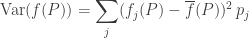
A good way to think about the Fisher speed is that it’s ‘the rate at which information is being updated’. A population of replicators of different species gives a probability distribution. Like any probability distribution, this has information in it. As the populations of our replicators change, the Fisher speed says the rate at which this information is being updated. So, in simple terms, we’ll show
The square of the rate at which information is updated is equal to the variance in fitness.
This is quite a change from Fisher’s original idea, namely:
The rate of increase of mean fitness is equal to the variance in fitness.
But it has the advantage of always being true… as long the population dynamics are described by the general framework we introduced last time. So let me remind you of the general setup, and then prove the result!
The setup
We start out with population functions 


for some differentiable functions 

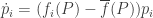
Using the Lotka–Volterra equation we showed last time that these probabilities obey the replicator equation

Here 
is the mean fitness.
The Fisher metric
The space of probability distributions on the set 

It’s called 


The Fisher metric is a Riemannian metric on the interior of the (n-1)-simplex. That is, given a point 


Here we are describing the tangent vectors 


If we have a probability distribution 

if the derivative 
Now we’ve got all the formulas we’ll need to prove the result we want. But for those who don’t already know and love it, it’s worthwhile saying a bit more about the Fisher metric.
The factor of 

But the reason the Fisher metric is important, I think, is its connection to relative information. Given two probability distributions 

You can show this is the expected amount of information gained if 
Suppose
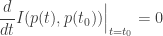
That is, in some sense ‘to first order’ no information is being gained at any moment 

So, the square of the Fisher speed has a nice interpretation in terms of relative entropy!
For a derivation of these last two equations, see Part 7 of my posts on information geometry. For more on the meaning of relative entropy, see Part 6.
The result
It’s now extremely easy to show what we want, but let me state it formally so all the assumptions are crystal clear.
Theorem. Suppose the functions 

for some differentiable functions 
Then if none of the populations 


Proof. The proof is near-instantaneous. We take the square of the Fisher speed:
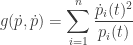
and plug in the replicator equation:
We obtain:

as desired. █
It’s hard to imagine anything simpler than this. We see that given the Lotka–Volterra equation, what causes information to be updated is nothing more and nothing less than variance in fitness!
The whole series:
• Part 1: the obscurity of Fisher’s original paper.
• Part 2: a precise statement of Fisher’s fundamental theorem of natural selection, and conditions under which it holds.
• Part 3: a modified version of the fundamental theorem of natural selection, which holds much more generally.
• Part 4: my paper on the fundamental theorem of natural selection.


Typo: You have a stray comma in the Lotka–Volterra equation (the first time).
This reminds me to remark that these generalized Lotka–Volterra equations hardly say anything more than that the quantities are governed by a system of time-independent differential equations at all. What they do say beyond that is that when
when  (and that any implicit continuity assumptions you make about the differential equations hold even more strongly at zero). This is quite reasonable, because if the population is zero at any time, then it can hardly change thereafter. But you only look in the interior where none of the
  are zero anyway, so now it says nothing extra again.
Yes, the Lotka–Volterra equations are scarcely more than the general system of first-order time-independent ODE! I should have said this. It’s interesting you can get anything out of them at all.
The main reason for writing
instead of
is that the functions do useful things for us when we bring in probabilities: their means, variances and such are interesting.
But it’s also important that the Lotka–Volterra equations imply that if vanishes at some time it vanishes at all later times (since I’m assuming the
  are differentiable—Lipschitz would be enough for this result). This means there’s “no true novelty”: no species can come into existence if it’s not there already. This means we’re not doing a full-fledged study of mutation. So we’re studying “natural selection” but not this other important aspect of evolution. (There are also lots of other aspects of evolution that we’re not getting into, of course.)
Similarly, any dynamic confined to the interior of the simplex is actually a replicator equation. This is called “forward-invariance”.
If a dynamic is forward-invariant on interior of the simplex, then we must have that
  since
since  . So we can rewrite the dynamic as follows:
which is a replicator equation with fitness functions .
.
AFAIK this was first noticed by Dashiell Fryer and myself [1] and [2]. It was also reported essentially as written above recently in [3], which notes a similar observation due to Smale in 1976 (before the common form of replicator equation was defined, typically attributed to Talyor and Jonker in 1978).
[1] Fryer (2012) On the existence of general equilibrium in finite games and general game dynamics. arXiv:1201.2384
[2] Harper, Fryer (2014). Lyapunov Functions for Time-Scale Dynamics on Riemannian Geometries of the Simplex, DGAA
[3] Raju, Krishnaprasad “Lie algebra structure of fitness and replicator control” (2020) arXiv:2005.09792
Off topic, but what is your take on the fact that a mathematical physicist has won the Nobel Prize for physics? Is that the first time that has happened? Actually, Penrose is a mathematician by training. (Fair enough I suppose since physicist Edward Witten, who also has a degree with a major in history and minor in linguistics and worked as a journalist and studied economics and maths for a while before coming to physics—not that it took long since he was a full professor at the IAS at Princeton at just barely 26—has won the Fields Medal.)
It seems strange that the acceleration of the information is equal to a squared speed. Since information is measured in bits, d²/dt² I is bits per second squared, which means the Fisher speed has units of “square root of bits” per second.
But is that meaningful? Think of something like flux density which is power per area per hertz. But since power is energy per time this is energy per area per time per hertz, but hertz has units of 1 over time so they cancel and we are left with energy per area which is formally correct in a sense but intuitively removed from the concept of flux density.
On a related note, power is energy per time and of course time is money and knowledge is power. Solving for money, we see that it diverges as knowledge goes to zero, regardless of the energy (e.g. tweeting) expended, which explains why Donald Trump earns more than I do. :-)
There must be a sign error somewhere; Trump is massively in debt.
Since bits are normally regarded as dimensionless this is tolerable, but I agree it’s strange. Fundamentally what’s strange is that as you start with and start moving
  away from
  the relative information
  doesn’t change to first order—only to second order! “To first order, you’re never learning anything”. So relative information is not like distance. It’s more like the square of distance.
But of course this follows from the fact that depends smoothly on
 and
and  when
when  A smooth nonnegative function that vanishes at some point must have vanishing derivative at that point. It can have nonvanishing second derivative, though!
And this is actually connected in a nice way to how distance is the square root of a fundamentally simpler quantity
John (if I may),
‘Fitness’ and ‘natural selection’ lead to the question, “What exactly is it, which has the fitness to be selected by nature?”
In the SEP article on fitness (https://plato.stanford.edu/entries/fitness/) there is some math and a section on “How the Problems of Defining Biological Individuality Affect the Notion of Fitness.” Here, the question of “What is it that’s fit?” raises a key issue in immunology. And then, a book is cited: “The Limits of the Self: Immunology and Biological Identity” by Thomas Pradeu.
The issue is how the immune systems knows to attack an ‘other,’ and when it overreacts (as sometimes in COVID) to attack its ‘self.’ Here is a review of The Limits of Self–
https://ndpr.nd.edu/news/the-limits-of-the-self-immunology-and-biological-identity/
This question is outside those addressed by Shannon-theoretic information. A different mathematics of information seems to be required. For example, say there is uncertainty among three possible entities within the detection process of the immune system: other1, other2, other3.
In Shannon’s theory of information, if any one of these three is ultimately detected, the amount of information (or ‘surprisal’) is the same. In this situation, Shannon’s theory makes no difference between other1, other2, or other3. The best text on this characteristic of Shannon information that I’ve read is by Fred Dretske– Chapter 1 of his book ‘Knowledge and the Flow of Information.’
Put another way, in this case, the problem for a mathematical theory of information is to detect the immunological ‘self.’ As well as others.
Now consider situation theory, channel theory, or ‘informationalism’ as introduced by Jon Barwise (the last, shortly before he passed away). My apologies for not formatting the math using latex. But here is some text on how that mathematical theory of information works to identify self and others:
First the self is a constituent of a situation. For example, say that along the lines of The Limits of Self, the self is a continuous process, symbolized in ordinary Petri nets by a transition (the continuous process), with one of its arrows pointed to a place labelled ‘self’ (a possibility), and then an arrow from that place back into the transition (the continuous process). This Petri net could symbolize the self inside its situation.
Now add an element of information (an ‘infon’) to this situation– that the self knows that it is in this situation in which it exists, or in which it occurs.
And then– if there are any others in this situation, by knowing the situation in which they, as well as its self, exist, it therefore knows them as well.
This machinery is detailed using mathematical symbols in Barwise’s Situation in Logic– in his chapter on common knowledge.
https://web.stanford.edu/group/cslipublications/cslipublications/site/0937073326.shtml
https://projecteuclid.org/euclid.ndjfl/1039540766