Last time we worked out an analogy between classical mechanics, thermodynamics and probability theory. The latter two look suspiciously similar:
| Classical Mechanics | Thermodynamics | Probability Theory | |
| q | position | extensive variables | probabilities |
| p | momentum | intensive variables | surprisals |
| S | action | entropy | Shannon entropy |
This is no coincidence. After all, in the subject of statistical mechanics we explain classical thermodynamics using probability theory—and entropy is revealed to be Shannon entropy (or its quantum analogue).
Now I want to make this precise.
To connect classical thermodynamics to probability theory, I’ll start by discussing ‘statistical manifolds’. I introduced the idea of a statistical manifold in Part 7: it’s a manifold 


Then I’ll talk about statistical manifolds of a special sort used in thermodynamics, which I’ll call ‘Gibbsian’, since they really go back to Josiah Willard Gibbs.

In a Gibbsian statistical manifold, for each

More precisely: in a Gibbsian statistical manifold we have a list of observables 


Statistical manifolds
Let’s fix a measure space 


and

for all

The idea here is that the space of all probability distributions on 
Information geometry is the geometry of statistical manifolds. Any statistical manifold comes with a bunch of interesting geometrical structures. One is the ‘Fisher information metric’, a Riemannian metric I explained in Part 7. Another is a 1-parameter family of connections on the tangent bundle 
• Hiroshi Matsuzoe, Statistical manifolds and affine differential geometry, in Advanced Studies in Pure Mathematics 57, pp. 303–321.
I don’t want to talk about it now—I just wanted to reassure you that I’m not completely ignorant of it!
I want to focus on the story I’ve been telling, which is about entropy. Our statistical manifold

namely
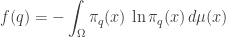
We can use this entropy function to do many of the things we usually do in thermodynamics! For example, at any point

which has an important physical meaning. In coordinates we have

and we call 

Defining 

of the cotangent bundle 


But I’ve been talking about these ideas for the last three episodes, so I won’t say more just now! Instead, I want to throw a new idea into the pot.
Gibbsian statistical manifolds
Thermodynamics, and statistical mechanics, spend a lot of time dealing with statistical manifold of a special sort I’ll call ‘Gibbsian’. In these, each probability distribution
How does this work? For starters, an integrable function

is called a random variable, or in physics an observable. The expected value of an observable is a smooth real-valued function on our statistical manifold

given by
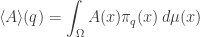
In other words, 

Now, suppose our statistical manifold is n-dimensional and we have n observables 
This may sound rather unlikely, but it’s really not so outlandish. Indeed, if there’s a point 

So, let’s assume the expected values of our observables give a coordinate system on 


Now for the kicker: we say our statistical manifold is Gibbsian if for each point
Which condition? The condition saying that
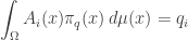
for all i. This is just the previous equation spelled out so that you can see it’s a condition on
This assumption of the entropy-maximizing nature of

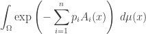
for all
Here 


By the way, this formula may look confusing at first, since the left side depends on the point
I’ll tell you: the conjugate variable 

and the evaluating this derivative at the point
But wait a minute! 
The entropy of 
So there’s something circular about our formula for
This is actually okay. While circular, the formula for
Next time I’ll prove that this formula for
• 

• 

• 

While these special cases are important and interesting, I’d rather be general!
Technical comments
I said “Any statistical manifold comes with a bunch of interesting geometrical structures”, but in fact some conditions are required. For example, the Fisher information metric is only well-defined and nondegenerate under some conditions on the map
Similarly, the entropy function
Furthermore, the integral
may not converge for all values of the numbers 
actually exists. In this case the probability distribution is also unique (almost everywhere).
For all my old posts on information geometry, go here:


Typos: You have a lot of unLaTeXed dollar signs in the last paragraph of the introduction and the first paragraph of the first section.
Whoops, and I was using some older notation I had for statistical manifolds. I fixed that. I’m trying to use for a statistical manifold now that I’m treating points
  as analogous to points in a ‘configuration space’ in classical mechanics. This goes against the conventions in Part 3, but I’ll deal with that in the unlucky event that I turn this stuff into a book.
I see, the introduction had all the wrong letters originally! There's still an unLaTeXed $q \in Q$ in the last paragraph of the introduction and an unLaTeXed $Omega,$ in the first paragraph of the first section.
I think there might be a typo at the end: “I was assuming that an entropy-minimizing probability distribution \pi_q “. Do you mean maximizing? In the integral coming right after, is A missing a subscript (this also occurs earlier)?
Also, could you please go a bit more into the definition of Gibbsian in your next installment? I’m not understanding what’s assumed and what’s implied by the condition.
Thanks!
Thanks for catching those mistakes. I tried to fix them.
What don’t you get about the definition of Gibbsian? I defined it precisely – or so I thought. You may not be familiar with Gibbs distributions, so maybe I need to explain something that seems obvious to me. But you have to tell me what you’re puzzled by! It’s hard to help without knowing what’s the problem.
What I mainly plan to do next time is prove that the Gibbs distribution
maximizes the entropy
subject to the constraints that
for all i.
I guess I’m confused about what the q_{i} are supposed to be: you defined them starting from A_{i} and the distribution, but now you use them to define another distribution. So do we assume that we have coordinates q_{i} on Q and observables A_{i} on \Omega already, and then consider probability distributions for which the expectatin of A_{i} is q_{i}?
Francis wrote:
No, there’s only one distribution in this story: or more precisely, one map sending each point
  of a manifold
  to a probability distribution
Starting from this and some observables I defined the function
to be the expected value of in the distribution
  :
:
Then I assumed that the functions are a coordinate system on
  (and I explained why this is easy to achieve).
Then I made a big extra assumption: is the probability distribution with the largest possible entropy such that
for all i. In other words: if you tell me the values of the coordinates then
then  is not just any old probability distribution having these values as the expected values of the observables
  It’s the probability distribution with the largest possible entropy having these values as the expected values of the observables
I’m not changing here, I’m just making an extra assumption about it. This is a common assumption in thermodynamics.
Without this extra assumption there’s nothing very exciting we can do until someone tells us a formula for . But with this extra assumption I can show that
  must obey this equation:
(I defined and
and  in the post.)
I will actually show this equation next time.
I hope the logic is clearer now. If there’s something puzzling still, just ask.
I added a bit about the traditional reasons for caring about Gibbsian statistical manifolds and the variables and
and  :
:
Great post! Question: what is the information analogue of FORCE?
Hi! That’s a good question. I will answer it someday, as I keep discussing the analogy between classical mechanics and information geometry. There are actually a few different possibilities, depending on what we take as the analogue of time.
It is pretty convoluted; I had to go through it a few times.
I think that it would help to use different symbols for (a point of the manifold
  ) and
) and  (a coordinate function on
  ). Because even though
  can be written as a tuple using the coordinates
  , still
  comes well before
  in the development.
Everyone in differential geometry uses as coordinates of a point called
  everyone in physics uses
  as coordinates of a position called
  etc. This is confusing when you first see it, and you might feel tempted to write
  for the coordinate function
  evaluated at the point
  But it’s good to get used to.
I’m sorry my exposition seemed convoluted. Maybe it’s because I was trying to explain two subjects in one blog post: statistical manifolds and thermodynamics. They’re closely related. In a statistical manifold each point labels a probability distribution. In thermodynamics each point of a manifold labels a probability distribution that maximizes entropy subject to constraints on some observables, and the expected values of these observables serve as coordinates.
I didn’t have a whole lot I wanted to say about statistical manifolds this time, except as a lead-in to thermodynamics. So I just laid out the basic formalism and then took a hard right turn into thermodynamics. If I ever turn this stuff into a book I’ll try to give the readers a more gentle ride.
Yes, but they do this when they start with the coordinates. Here the coordinates are derived at the end of a series of steps; I think that's adding to the confusion. I see why you did it this way, but it is an unusual order to do things.
Anyway, I'm really hoping that people who see these comments might think ‹Ah, that's why I'm confused, but now I understand.› rather than that you'll change the notation, especially since I don’t have a natural alternative to suggest.
Yeah. Socrates once complained that the problem with books is that you can’t ask a book questions. But on a blog you can ask questions — and other people can read the answers! This is what I like about blogs.
You might like
https://www.annualreviews.org/doi/full/10.1146/annurev-statistics-060116-054026
esp Fig 1.
That’s interesting, but I’m suspicious of it for some reason.