
I love this movie showing a solution of the Kuramoto–Sivashinsky equation, made by Thien An. If you haven’t seen her great math images on Twitter, check them out!
I hadn’t known about this equation, and it looked completely crazy to me at first. But it turns out to be important, because it’s one of the simplest \partial differential equations that exhibits chaotic behavior.
As the image scrolls to the left, you’re seeing how a real-valued function 


Near the end of this post I’ll make some conjectures about the Kuramoto–Sivashinsky equation. The first one is very simple: as time passes, stripes appear and merge, but they never disappear or split.
The behavior of these stripes makes the Kuramoto–Sivashinsky equation an excellent playground for thinking about how differential equations can describe ‘things’ with some individuality, even though their solutions are just smooth functions. But to test my conjectures, I could really use help from people who are good at numerical computation or creating mathematical images!
First let me review some known stuff. You can skip this and go straight to the conjectures if you want, but some terms might not make sense.
Review
For starters, note that these stripes seem to appear out of nowhere. That’s because this system is chaotic: small ripples get amplified. This is especially true of ripples with a certain wavelength: roughly 
And yet while solutions of the Kuramoto–Sivanshinsky equation are chaotic, they have a certain repetitive character. That is, they don’t do completely novel things; they seem to keep doing the same general sort of thing. The world this equation describes has an arrow of time, but it’s ultimately rather boring compared to ours.
The reason is that all smooth solutions of the Kuramoto–Sivanshinsky equation quickly approach a certain finite-dimensional manifold of solutions, called an ‘inertial manifold’. The dynamics on the inertial manifold is chaotic. And sitting inside it is a set called an ‘attractor’, which all solutions approach. This attractor is probably a fractal. This attractor describes the complete repertoire of what you’ll see solutions do if you wait a long time.
Some mathematicians have put a lot of work into proving these things, but let’s see how much we can understand without doing anything too hard.
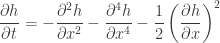
Written out with a bit less jargon, the Kuramoto–Sivashinky equation says
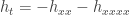
or in more compressed notation,

To understand it, first remember the heat equation:

This describes how heat spreads out. That is: if 

But the Kuramoto–Sivashinsky equation more closely resembles the time-reversed heat equation

This equation describes how, running a movie of a hot iron rod backward, heat tends to bunch up rather than smear out! Small regions of different temperature, either hotter or colder than their surroundings, will tend to amplify.
This accounts for the chaotic behavior of the Kuramoto–Sivashinsky equation: small stripes emerge as if out of thin air and then grow larger. But what keeps these stripes from growing uncontrollably?
The next term in the equation helps. If we have
then very sharp spikes in
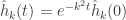
To see this, it helps to bring in a bit more muscle: Fourier series. We can easily solve the heat equation if our iron rod is the interval ![[0,2\pi]](https://s0.wp.com/latex.php?latex=%5B0%2C2%5Cpi%5D&bg=ffffff&fg=333333&s=0&c=20201002)

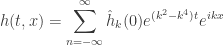
This lets us write the temperature function 

for some functions 

and we can easily solve these equations and get
and thus

So, each function 

If we solve the time-reversed heat equation the same way we get

so now high-frequency modes get exponentially amplified. The time-reversed heat equation is a very unstable: if you change the initial data a little bit by adding a small amount of some high-frequency function, it will make an enormous difference as time goes by.
What keeps things from going completely out of control? The next term in the equation helps:
This is still linear so we can still solve it using Fourier series. Now we get

Since 

We can make the story more interesting if we don’t require our rod to have length 

![[0,L]](https://s0.wp.com/latex.php?latex=%5B0%2CL%5D&bg=ffffff&fg=333333&s=0&c=20201002)


for integers 
but we have to remember 


If 


Which exponentially growing modes grow the fastest? These are the ones that make 

namely 


In short, our equation has a certain length scale where the instability is most pronounced: temperature waves with about this wavelength grow fastest.
All this is very easy to work out in as much detail as we want, because our equation so far is linear. The full-fledged Kuramoto–Sivashinsky equation
is a lot harder. And yet some features of the linear version remain, which is why it was worth spending time on that version.
For example, I believe the stripes we see in the movie above have width roughly 

• Encyclopedia of Mathematics, Kuramoto–Sivashinsky equation.
The inertial manifold
The most fascinating fact about the Kuramoto–Sivashinsky equation is that for any fixed length 

As I mentioned, the manifold
• Wikipedia, Inertial manifold.
To make these ideas precise we need to choose a notion of distance between two solutions at a given time. A good choice uses the 

Functions on ![L^2[0,L]](https://s0.wp.com/latex.php?latex=L%5E2%5B0%2CL%5D&bg=ffffff&fg=333333&s=0&c=20201002)


• P. Collet, J.-P. Eckmann, H. Epstein and J. Stubbe, Analyticity for the Kuramoto–Sivashinsky equation, Physica D 67 (1993), 321–326.
This smoothing property is well-known for the heat equation, but it’s much less obvious here!
This work also shows that the Kuramoto–Sivashinsky equation defines a dynamical system on the Hilbert space

• Roger Temam and Xiao Ming Wang, Estimates on the lowest dimension of inertial manifolds for the Kuramoto-Sivashinsky equation in the general case, Differential and Integral Equations 7 (1994), 1095–1108.
I conjecture that in reality its dimension grows roughly linearly with 


This evidence is rather weak, since it completely ignores the nonlinearity of the Kuramoto–Sivashinsky equation. I would not be shocked if the dimension of the inertial manifold grew at some other rate than linearly with
Sitting inside the inertial manifold is an attractor, the smallest set that all solutions approach. This is probably a fractal, since that’s true of many chaotic systems. So besides trying to estimate the dimension of the inertial manifold, which is an integer we should try to estimate the dimension of this attractor, which may not be an integer!
There have been some nice numerical experiments studying solutions of the Kuramoto–Sivashinsky equation for various values of
• Demetrios T. Papageorgiou and Yiorgos S. Smyrlis, The route to chaos for the Kuramoto–Sivashinsky equation, Theoretical and Computational Fluid Dynamics 3 (1991), 15–42.
I’ll warn you that they use a slightly different formalism. Instead of changing the length

for some number 
Conjectures
There should be some fairly well-defined notion of a ‘stripe’ for the Kuramoto–Sivashinsky equations: you can see the stripes form and merge here, and if we can define them, we can count them and say precisely when they’re born and when they merge:
For now I will define a ‘stripe’ as follows. At any time, a solution of the Kuramoto–Sivashinsky gives a periodic function 
![[0,L].](https://s0.wp.com/latex.php?latex=%5B0%2CL%5D.&bg=ffffff&fg=333333&s=0&c=20201002)


So, here are the conjectures:
First, I conjecture that if 
(Here ‘almost every’ is in the usual sense of measure theory. There are certainly solutions of the Kuramoto–Sivashinsky equation that don’t have stripes that appear and merge, like constant solutions. These solutions may lie on the inertial manifold, but I’m claiming they are rare.)
I also conjecture that the time-averaged number of stripes is asymptotically proportional to 
I also conjecture that there’s a well-defined time average of the rate at which new stripes form, which is also asymptotically proportional to
I also conjecture that this rate equals the time-averaged rate at which stripes merge, while the time-averaged rate at which stripes disappear or split is zero.
These conjectures are rather bold, but of course there are various fallback positions if they fail.
How can we test these conjectures? It’s hard to explicitly describe solutions that are actually on the inertial manifold, but by definition, any solution keeps getting closer to the inertial manifold at an exponential rate. Thus, it should behave similarly to solutions that are on the inertial manifold, after we wait long enough. So, I’ll conjecture that the above properties hold not only for almost every solution on the inertial manifold, but for typical solutions that start near the inertial manifold… as long as we wait long enough when doing our time averages.
If you feel like working on this, here are some things I’d really like:
• Images like Thien An’s but with various choices of 

and run it for long enough to ‘settle down’—that is, get near the inertial manifold.
• A time-averaged count of the average number of stripes for various choices of
• Time-averaged counts of the rates at which stripes are born, merge, split, and die—again for various choices of
If someone gets into this, maybe we could submit a short paper to Experimental Mathematics. I’ve been browsing papers on the Kuramoto–Sivashinsky equations, and I haven’t yet seen anything that gets into as much detail on what solutions look like as I’m trying to do here.
The arrow of time
One more thing. I forgot to emphasize that the dynamical system on the Hilbert space
What makes this especially interesting is that the dynamical system on the inertial manifold probably is reversible. As long as this manifold is compact, it must be: any smooth vector field on a compact manifold
And yet, even if this flow is reversible, as I suspect it is, it doesn’t resemble its time-reversed version! It has an ‘arrow of time’ built in, since bumps are born and merge much more often than they merge and split.
So, if my guesses are right, the inertial manifold for the Kuramoto–Sivashinsky equation describes a deterministic universe where time evolution is reversible—and yet the future doesn’t look like the past, because the dynamics carry the imprint of the irreversible dynamics of the Kuramoto–Sivashinsky equation on the larger Hilbert space of all solutions.
A warning
If you want to help me, the following may be useful. I believe the stripes are ‘bumps’, that is, regions where 


Here the stripes are not mere bumps: they are regions where, as we increase
After massive confusion I realized that Steve was using some MATLAB code adapted from this website:
• Mathab Lak, Test case for PDEs: Kuramoto–Sivashinksy, Crank-Nicolson/Adams-Bashforth (CNAB2) timestepping.
and this code solves a different version of the Kuramoto–Sivashinksy equations, the so-called derivative form:

If
then its derivative

satisfies the derivative form.
So, the two equations are related, but you have to be careful because some of their properties are quite different! For the integral form, the cross-section of a typical stripe looks very roughly like this:
.jpg)
but for the derivative form it looks more like this:

You can grab Steve Huntsman’s MATLAB code here, but beware: this program solves the derivative form! Many of Steve’s pictures in comments to this blog—indeed, all of them so far—show solutions of the derivative form. In particular, the phenomenon he discovered of stripes tending to move at a constant nonzero velocity seems to be special to the derivative form of the Kuramoto–Sivashinsky equation. I’ll say more about this next time.


Amazing. But what happens if we convert this to a difference equation? Might better show the chaotic property? http://www.math-math.com/2018/02/the-calculus-that-got-ignored.html
I don’t see why it would be any ‘better’, but when you numerically solve this differential equation, e.g. using the Euler method or Runge–Kutta, you’re implicitly turning it into a difference equation. And by the way, the fact that the original equation is chaotic means that your numerical solution will be unstable: small errors will blow up. You just have to live with that and hope that if you do a decent job, they won’t affect the ‘overall character’ of the solutions (e.g. the properties I’m conjecturing).
I wonder how much of the behavior you could replicate with a three value function, i.e by describing things at the level of “things” and ignoring the smooth foundation. Like if all you know about a point is if it’s blue yellow or green (low high middle) can you predict the future? I kind think you should be able to recover the continuous function.
And then of course the the other question is how many computational pixels do you need per bump? 2 5 10 1?
Good questions! I bet there are quite simple cellular automaton models that display behavior similar to the Kuramoto–Sivashinsky equation. Does someone here know them?
There are lattice Boltzmann models, e.g. https://doi.org/10.1016/j.physa.2009.01.005 but these sorts of things are rather more involved than cellular automata per se. I once tinkered with such things and the effort is almost all technicalities (of the sort I find annoying)
I think it might be hard to find a threshold c for defining bumps. In the video, it appears to me that just before bumps merge, they sometimers get pinched, or fade away a bit, especially if they are ‘young’ bumps, not well established ones. The Encyclopedia of Mathematics link has a ‘derivative’ version which looks symmetric about zero, so perhaps a threshold of zero would work for that.
If you look at the valleys instead of the bumps, they tend to split and die, not emerge and merge. That is more like how life works. I like to think of the bumps as reproductive barriers between species.
I was confused about how to read this image:
I thought the stripes were ‘bumps’: regions where for some positive
  In fact the light side of each stripe has
  and the dark side has
  (or maybe the other way around). In other words, brightness is proportional to
This was clarified by Steve Huntsman, who produced an image showing the actual value of
So, I need to define stripes correctly to fix my conjectures.
Of course if I can define which regions are in stripes, I can define which regions are not in stripes.
Note that it takes to about for the solution to come close to the inertial manifold. For about
  small initial ripples are merging and growing to form a few big stripes. By about
  we see the usual pattern: stripes merging and being born at a roughly constant rate.
By the way, the values on Steve Huntsman’s image seem awfully large to me. Maybe they’re rescaled somehow? I may need to learn to write my own programs for this stuff.
(Note added later: some of the confusion above is cleared up in the current version of the blog article, written 2021 October 21.)
Maybe Greg Egan might be interested in helping? He’s got some sophisticated animations on his website. Or maybe Grant Sanderson might be interested. Either might be willing to share or point to some useful animation tools.
I was confused in the same way as you… unless people are using different definitions of u.
In Steve Huntsman’s image, I’d be inclined to find zero-crossings and remove those that cross zero ‘too gently’. This is aimed at defining borders rather than regions.
Yes, my article here discusses what the Encyclopedia of Mathematics calls the ‘derivative’ form of the equation, while they mainly discuss the ‘integral’ form. You get a solution of the derivative form by differentiating a solution of the integral form with respect to
Since Thien An showed the derivative form on her movie, I optimistically assumed she was working with that form.
However, this code claims to be solving the integral form.
This makes a difference in how to define ‘stripes’, and right now I’m rather confused.
Steve Huntsman claims to be solving the derivative form and getting this:
Maybe this is why people program: if you don’t do the programming yourself you can never feel sure about what’s actually happening. Unfortunately, when I program myself I still can’t tell what’s actually happening.
Ha! I didn’t write the code myself so I don’t understand what’s happening either, just taking the code comment at face value. But it wouldn’t be that hard to rewrite/understand it…
I had no idea this sort of behaviour could arise from a differential equation, it’s extremely beautiful.
I wonder if there is a straightforward 3d generalization where the bumps braid around each other before merging.
Yes! I didn’t say it out loud, but here’s what we’re both thinking.
If you have a monoid object in a monoidal category, it has a multiplication
and unit
and if we draw morphisms involving these as string diagrams, we get 2-dimensional pictures where strings can merge (thanks to the multiplication) and be born (thanks to the unit), but never split or die.
Braiding might be possible in this ‘chemotaxis’ model animated by Theodore Kolokolnikov:
But actually I don’t see braiding going on here. Maybe the ‘bacteria’ need more freedom to randomly roam about if you want braiding to happen.
Theodore Kolokolnikov made some interesting comments in email, which he’s letting me post here:
Here is a version Steve Huntsman did with Here time goes across the page. You can click to enlarge it. Note that the solution is close to spatially periodic until about
  because the initial conditions are periodic, but then chaos starts to take over and it destroys the periodicity:
Steve Huntsman wrote:
I’ve updated the code and am close enough to grokking it that I believe it is correct or else there’s a Wikipedia conspiracy on the numerical integration scheme pages (since I haven’t dug into these or done Crank-Nicolson since 1998).
Using this and running
Lx = 128;
Nx = 1024;
dt = 1/16;
Nt = 1600;
%
x = Lx*(0:(Nx-1))/Nx;
u = cos(x) + 0.1*cos(x/16).*(1+2*sin(x/16));
%
[U,x,t] = kuramotoShivashinskyIntegrate(u,Lx,dt,Nt);
figure;
%
subplot(1,2,1);
pcolor(x,t,real(U));
shading interp;
xlabel(‘$x$’,’Interpreter’,’latex’);
ylabel(‘$t$’,’Interpreter’,’latex’);
%
subplot(1,2,2);
plot(sum(abs(diff(sign(real(U)),1,2)),2)/4,t,’k’);
xlabel(‘number of stripes’,’Interpreter’,’latex’);
ylabel(‘$t$’,’Interpreter’,’latex’);
yields
(Note that you can count the t = 0 and t = 100 stripes to confirm the plot on the right.) All the number of stripes counts is the zero crossings as in the blog comments. I see no reason to limit this to something “sufficiently large.”
Great! So, just eyeballing it, after the stripe count settles down to its average, we’re getting about 15 stripes when L = 128, for an average density of about 15/128 1/8.5.
I’m predicting this stripe density approaches a constant that’s indepdent of the initial data as we time-average over longer and longer times, and that this constant in turn approaches a limit as L
Steve Huntsman writes:
Using initial conditions where the initial conditions at each grid point is IID uniform on [0,1], here’s 3 realizations:
(There’s a new kind of symmetry breaking?) Running longer:
Taking initial conditions cos(x)+0.1*IID uniform on [0,1]:
Seems like the lucky number for L = 128 is ~14 stripes. I may come back to this tomorrow.
This is fascinating. Here’s the thing that may force me to change my conjectures:
All the stripes seem to be moving to the left as time passes!
There could be some conserved quantity like ‘momentum’ for this differential equation—conserved despite the chaos!—and if so, the inertial manifold does not contain a single attractor, but a family parametrized by momentum. If so, we can’t expect all solutions to have the same time-averaged properties. These properties can depend on the momentum.
Or maybe something else is going on. What’s weird is that all three solutions with i.i.d. random initial conditions have stripes strongly moving to the left! That’s a real shocker.
By the way, this is related to the question of a conserved momentum. The Encyclopedia of Mathematics article writes this about the Kuramoto–Sivashinsky equation:
The translational symmetry of the equation is obvious, and if the equations come from a Lagrangian this symmetry will give a conserved momentum by Noether’s theorem. But the heat equation does not come from a Lagrangian, so it does not have a conserved momentum. I’m afraid the Kuramoto–Sivashinsky equation is similar. But I’m not sure.
The Galilean symmetry is surprising to me. In fact it’s hard to believe. This would mean we can ‘boost’ a solution and get a new solution that’s moving relative to the original one. That’s not true of the heat equation!
The parity symmetry makes me shocked that in so many of these solutions, all the stripes have u > 0 on the same side.
It seem that there are the attractors
that are invariant functions, but I don’t find the analytic solution, only the trivial solution u=constant; but exist functions that are time invariants.
Solutions near to the attractors should be close in the initial instants of motion.
One paper I read said there are no known analytical solutions of the closely related equation
except for zero of course, but they were nonetheless able to prove a lot about periodic-in-space solutions of this equation:
• Uriel Frisch, Zhensu She and Olivier Thual, Viscoelastic behaviour of cellular solutions to the Kuramoto–Sivashinsky model, Journal of Fluid Mechanics 168 (1986), 221–240.
Well IID uniform on [0,1] is different than IID on [-1,1]. My money is on that as the culprit for the “momentum”. Stay tuned this evening
Steve wrote:
Earlier I had guessed ~15, just by eyeballing one of your pictures. So now we’re getting a stripe density of about 14/128 1/9.14.
It’s not at all obvious why this should also be true of solutions where the stripes ‘slant’ a lot, as in some of your recent pictures. If the stripe density is really the same for these that seems like a nontrivial fact. But I’m quite puzzled by what’s going on in these slanted solutions.
Today (2021 October 21) I rewrote this blog post, correcting a bunch of errors that stemmed from me not realizing there are two different versions of the Kuramoto–Sivashinsky equation. If you care, and you read this article before today, you might like a look at the new version!
You are so conscientious John. In fact you’re one of the people I don’t know well who ranks highest in my ‘what would the world be like if X were generically median’ ranking. (I suspect professional sports might take it in the shorts, but I might be wrong & in any case that’s a tradeoff I’m willing to make😊)
Thanks! I don’t feel especially conscientious, but when I’m enthusiastic about something I care about it a lot.
Inspired by your post, I constructed an electric circuit equivalent for the Kuramoto Sivashinsky equation (derivative form), as shown here:
The R1 and R2 resistors encode the 2nd and 4th x-derivative. (The R1 are negative!). The R3 are non-linear, proportional to the gradient, or equivalently the currents in R1 and R2.
I can recreate the stripe patterns. But by accident, I initialized a case that converges to a regular stripe pattern! Shown here:
I used L=100, and the initial state was a sine-wave with 3 periods in L=100.
If on the other hand I initialize with some random numbers, I get the same kind of strips as in other posts:
Cool! For periodic boundary conditions with (spatial) period L, static stripe solutions are stable for small L, but for larger L they become unstable.
Let’s see how easy it is to link to your tweet:
Very fun write up! A small, possibly off-base, comment: these figures remind me of phase dislocations (Nye & Berry 1974: see also this paper: https://www.sciencedirect.com/science/article/abs/pii/0167278992900014). In the linked paper, some calculus constraining the topology of lines of constant phase can help us keep track of “wave” creation/annihilation and one can possibly estimate all kinds of useful statistical characterizations of the behavior of the stripes.
That sounds interesting! It’s a hassle to use the VPN client to be able to read this paper, and it doesn’t seem to be free anywhere, but I’ll give it a try sometime. There is an interesting comparison of the nonlinear stabilization mechanisms in the Kuramoto–Sivashinsky and Ginzburg–Landau equations on the second page here:
• P. Collet, J. Eckmann and J. Stubbe, A global attracting set for the Kuramoto–Sivashinsky equation, Communications in Mathematical Physics 152 (1993), 203–214.
They explain why Kuramoto–Sivashinsky is subtler.
[…] I had a passing read over a series of posts on Azimuth starting with this one, on one of the simplest ODEs that demonstrates chaotic behaviour. The timing of this series of […]