In my first post in this series, we saw that filling in a well-known analogy between statistical mechanics and quantum mechanics requires a new concept: ‘quantropy’. To get some feeling for this concept, we should look at some examples. But to do that, we need to develop some tools to compute quantropy. That’s what we’ll do today.
All these tools will be borrowed from statistical mechanics. So, let me remind you how to compute the entropy of a system in thermal equilibrium starting if we know the energy of every state. Then we’ll copy this and get a formula for the quantropy of a system if we know the action of every history.
Computing entropy
Everything in this section is bog-standard. In case you don’t know, that’s British slang for ‘extremely, perhaps even depressingly, familiar’. Apparently it rains so much in England that bogs are not only standard, they’re the standard of what counts as standard!
Let 

where of course

The entropy of this probability distribution is

There’s a nice way to compute the entropy when our system is in thermal equilibrium. This idea makes sense when we have a function

saying the energy of each state. Our system is in thermal equilibrium when 

A famous calculation shows that thermal equilibrium occurs precisely when

for some real number 


The number

where 
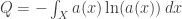
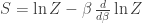
There’s a famous way to compute the entropy of the Gibbs state; I don’t know who did it first, but it’s both straightforward and tremendously useful. We take the formula for entropy
and substitute the Gibbs state
getting

Reshuffling this a little bit, we obtain:

If we define the free energy by

then we’ve shown that

This justifies the term ‘free energy’: it’s the expected energy minus the energy in the form of heat, namely

It’s nice that we can compute the free energy purely in terms of the partition function and the temperature, or equivalently the coolness

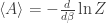
Can we also do this for the entropy? Yes! First we’ll do it for the expected energy:

This gives

So, if we know the partition function of a system in thermal equilibrium as a function of the temperature, we can work out its entropy, expected energy and free energy.
Computing quantropy
Now we’ll repeat everything for quantropy! The idea is simply to replace the energy by action and the temperature 

It’s annoying that in physics 


Let

where perhaps surprisingly

The quantropy of this function is
There’s a nice way to compute the entropy in Feynman’s path integral formalism. This formalism makes sense when we have a function

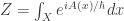
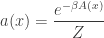
saying the action of each history. Feynman proclaimed that in this case we have

where
Last time I showed that we obtain Feynman’s prescription for 

subject to a constraint on the expected action:
As I mentioned last time, the formula for quantropy is dangerous, since we’re taking the logarithm of a complex-valued function. There’s not really a ‘best’ logarithm for a complex number: if we have one choice we can add any multiple of 


Luckily, the ambiguity is much less when we use Feynman’s prescription for 

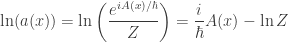
Once we choose a logarithm for
So let’s do this, and say the quantropy is
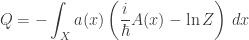
We can simplify this a bit, since the integral of

Reshuffling this a little bit, we obtain:
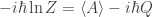
By analogy to free energy in statistical mechanics, let’s define the free action by

I’m using the same letter for free energy and free action, but they play exactly analogous roles, so it’s not so bad. Indeed we now have

which is the analogue of a formula we saw for free energy in thermodynamics.
It’s nice that we can compute the free action purely in terms of the partition function and Planck’s constant. Can we also do this for the quantropy? Yes!
It’ll be convenient to introduce a parameter

which is analogous to ‘coolness’. We could call it ‘quantum coolness’, but a better name might be classicality, since it’s big when our system is close to classical. Whatever we call it, the main thing is that unlike ordinary coolness, it’s imaginary!
In terms of classicality, we have
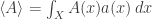
Now we can compute the expected action just as we computed the expected energy in thermodynamics:

This gives:

So, if we can compute the partition function in the path integral approach to quantum mechanics, we can also work out the quantropy, expected action and free action!
Next time I’ll use these formulas to compute quantropy in an example: the free particle. We’ll see some strange and interesting things.
Summary
Here’s where our analogy stands now:
| Statistical Mechanics | Quantum Mechanics |
states:  |
histories: |
probabilities:  |
amplitudes:  |
energy:  |
action:  |
| temperature: |
Planck’s constant times i: |
coolness:  |
classicality:  |
partition function: 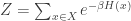 |
partition function:  |
Boltzmann distribution:  |
Feynman sum over histories:  |
entropy:  |
quantropy:  |
expected energy:  |
expected action:  |
free energy:  |
free action:  |
 |
 |
 |
|
 |

|
I should also say a word about units and dimensional analysis. There’s enormous flexibility in how we do dimensional analysis. Amateurs often don’t realize this, because they’ve just learned one system, but experts take full advantage of this flexibility to pick a setup that’s convenient for what they’re doing. The fewer independent units you use, the fewer dimensionful constants like the speed of light, Planck’s constant and Boltzmann’s constant you see in your formulas. That’s often good. But here I don’t want to set Planck’s constant equal to 1 because I’m treating it as analogous to temperature—so it’s important, and I want to see it. I’m also finding dimensional analysis useful to check my formulas.
So, I’m using units where mass, length and time count as independent dimensions in the sense of dimensional analysis. On the other hand, I’m not treating temperature as an independent dimension: instead, I’m setting Boltzmann’s constant to 1 and using that to translate from temperature into energy. This is fairly common in some circles. And for me, treating temperature as an independent dimension would be analogous to treating Planck’s constant as having its own independent dimension! I don’t feel like doing that.
So, here’s how the dimensional analysis works in my setup:
| Statistical Mechanics | Quantum Mechanics |
| probabilities: dimensionless | amplitudes: dimensionless |
energy:  |
action:  |
| temperature: |
Planck’s constant: |
coolness:  |
classicality:  |
| partition function: dimensionless | partition function: dimensionless | entropy: dimensionless | quantropy: dimensionless |
| expected energy: |
expected action: |
| free energy: |
free action: |
I like this setup because I often think of entropy as closely allied to information, measured in bits or nats depending on whether I’m using base 2 or base e. From this viewpoint, it should be dimensionless.
Of course, in thermodynamics it’s common to put a factor of Boltzmann’s constant in front of the formula for entropy. Then entropy has units of energy/temperature. But I’m using units where Boltzmann’s constant is 1 and temperature has the same units as energy! So for me, entropy is dimensionless.


“Feynman proclaimed that in this case we have…” two s that we said were to be
  !
!
Fixed!
I think it’s a mistake to say is analogous to T; it’s much more like Boltzmann’s constant k, a constant that’s there just to make the units work. It makes more sense to introduce a unitless parameter
  to play the role of temperature and have kT (with units of energy) analogous to
  (with units of action).
That sounds good, but what’s the physical meaning of ? Maybe it’s a dimensionless version of an adjustable Planck’s constant, with the original
  now playing the role of an arbitrary constant for the purposes of changing units?
The real physical problem is that in reality we can change the temperature but not .
.
Lambda’s a measure of classicality; it changes with the constraint on the expected action. By increasing the frequency of a particle (whether due to a photon’s momentum or a particle’s mass), the action along the path increases. For a particle of mass m, we can take to be m over the Planck mass.
Okay, this is getting good. Here’s another idea. When dealing with entropy we are doing integrals over states; when dealing with quantropy we are doing integrals over histories. Histories often have a built-parameter that states don’t: how long the history lasts. For example, for a particle moving on a line, a history is a path
so we have this parameter at hand. This parameter has dimensions of time, obviously. If we try to make this parameter go away by taking
  , we get nonsense because the action of most histories becomes infinite. So we need
  , and it’s probably good to make it explicit.
I noticed this while calculating the quantropy of a free particle.
So: in statistical mechanics we can adjust the temperature, but not really Boltzmann’s constant. In quantum mechanics we can adjust the length of time our histories last, but not really Planck’s constant. This seems like a promising analogy, especially since we’ve already thought about a famous analogy relating temperature to imaginary time.
This extra parameter is closely related to how action has units of energy × time. I think it should explain all the ‘discrepancies’ in units here:
Finally, I can’t resist adding that one of Hawking’s famous calculations of black hole entropy treat the coolness as how long the universe lasts in imaginary time.
(If you click the link I hope you get taken to page 47 of Hawking and Penrose’s book The Nature of Space and Time. This portion of this book written by Hawking is truly wonderful introduction to black hole thermodynamics and the concept of imaginary time. I recommend it to everyone who knows enough physics to understand, say, this blog entry. It’s accurate and meaty without becoming extremely technical. It explains what Hawking was actually thinking when he did his most famous work.)
What if you associate with your histories an energy and a “temperature”
  ?
?
That sounds interesting. I’d call your quantity
‘action per time’, or activity, or something. I will investigate these different options soon. It may be more fun after I explain an example of the formalism, namely the free particle. Then we can get more of a feeling for these concepts.
By the way, this business about ‘action = energy × time’ is closely related to Blake Stacey’s observation that in classical mechanics, conjugate quantities multiply to give something with units of action, while in thermodynamics, they multiply to give something with units of energy. This should ultimately resolve the puzzle of ‘if we try to quantize thermodynamics, what takes the place of Planck’s constant?’… though I can say I see how yet.
I like that idea even better. What both of them have in common is that lambda is the ratio of the time traversing the path to the time for a complete quantum vibration.
This is related to the ability to accurately determine the pitch of a note: it’s much more important to get your fingers in exactly the right place when you’re bowing a bass than when you’re plucking it.
It’s also related to the variant of Heisenberg’s inequality , where we have an observable Q that does not commute with the Hamiltonian and we define
  to be the time that it takes the expected value of Q to change by one standard deviation.
I notice the T versus T² in the dimensions. This reminds me of how thermodynamics uses the heat equation and quantum mechanics uses the wave equation, the difference between which is ∂/∂t versus (∂/∂t)². Except that it’s backwards!
Hmm, what if I say quantum mechanics uses the Schrödinger equation?
Schroedinger equation is more like a Wick rotated heat equation.
Just for fun. Bog standard was a standard phrase in Lancashire, UK at least from the 1960s.
One meaning of bog has always been a synonym for toilet in my experience of common english parlance.
Iiuc the US equivalent is “brown bag”.
Wiktionary has:
“Believed to derive from early ceramic toilets being produced to exactly the same specification in white only which became known as the bog standard. [1] [2]”
http://bit.ly/y2sbYW
Much enjoyed quantropy part 1. Thanks.
Thanks! I didn’t really believe in my folk etymology of ‘bog standard’, but I hoped my joke would elicit more accurate information. It’s interesting that ‘bog’ is a synonym for ‘toilet’. I’m (again somewhat jokingly) imagining that this goes back to primitive Anglo-Saxon customs.
I hope you liked part 2, too.
Funny, I heard a different and interesting etymology (probably from QI). Old (Hornby?) train sets used to come in two versions which were written ‘box standard’ and ‘box deluxe’, these were so so common that they got converted and distorted into the negative and positive phrases: ‘bog standard’ and ‘the dog’s bollocks’.
I’ve been talking a lot about ‘quantropy’. Last time we figured out a trick for how to compute it starting from the partition function of a quantum system. But it’s hard to get a feeling for this concept without doing some examples […]
If you have carefully read all my previous posts on quantropy (Part 1, Part 2 and Part 3), there’s only a little new stuff here. But still, it’s better organized […]
Besides questions, I like ‘analogy charts’, consisting of two or more columns with analogous items lined up side by side. You can see one near the bottom of my 2nd article on quantropy. Quantropy is an idea born of the analogy between thermodynamics and quantum mechanics […]
I really like ‘analogy charts’ with two or more columns, with analogous items lined up side by side. You can see one near the bottom of my 2nd article on quantropy. Quantropy is an idea born of the analogy between thermodynamics and quantum mechanics. […]