ACT2023 – Network Theory Talks

It’s not too late to register to join talks on Zoom at Applied Category Theory 2023. It starts on Monday July 31, 2023! But if you miss out, you can watch talks later on YouTube.

Here’s where you can register:

https://www.eventbrite.com/e/applied-category-theory-2023-registration-643212404617

and here’s the program of talks:

https://act2023.github.io/programme.html

Besides talks there will also be tutorials:

Monday (simultaneously):
• David Jaz Myers, Lenses
• Paolo Perrone, Markov categories
Tuesday (simultaneously):
• Dorette Pronk, Double categories
• Evan Patterson and Owen Lynch, AlgebraicJulia

The conference is big, so let me just point out a few talks connected to network theory.

I’ll talk about “Software for compositional modeling in epidemiology”. This project uses software based on category theory to make it easier to assemble big models of infectious disease—but our techniques work for other applications too. We’re using AlgebraicJulia, a computing framework based explicitly on categories—so check out the tutorial on that.

Some talks are based on work at last summer’s American Mathematical Society research program. For example James Fairbanks is talking about “A compositional account of motifs, mechanisms, and dynamics in biochemical regulatory networks” and Sophie Libkind is speaking on “Additive invariants of open Petri nets”, both based on projects I suggested there.

Also, Evan Patterson is giving a talk on “Structured and decorated cospans from the viewpoint of double category theory”, which may give new ideas for how AlgebraicJulia should handle networks. And if you don’t already know about double categories, Dorette Pronk’s tutorial should help.

A lot of good stuff!

Categories for Epidemiology

Xiaoyan Li, Sophie Libkind, Nathaniel D. Osgood, Eric Redekopp and I have been creating software for modeling the spread of disease… with the help of category theory!

Lots of epidemiologists use “stock-flow diagrams” to describe ordinary differential equation (ODE) models of disease dynamics. We’ve created two tools to help them.

The first, called StockFlow.jl, is based on category theory and written in AlgebraicJulia, a framework for programming with categories that many people at or associated with Topos have been developing. The second, called ModelCollab, runs on web browsers and serves as a graphical user interface for StockFlow.jl.

Using ModelCollab requires no knowledge of Julia or category theory! This feature should be useful in “participatory modeling”, an approach where models are built with the help of diverse stakeholders. However, as we keep introducing new features in StockFlow.jl, it takes time to implement them in ModelCollab.

But what’s a stock-flow diagram, and what does our software let you do with them?

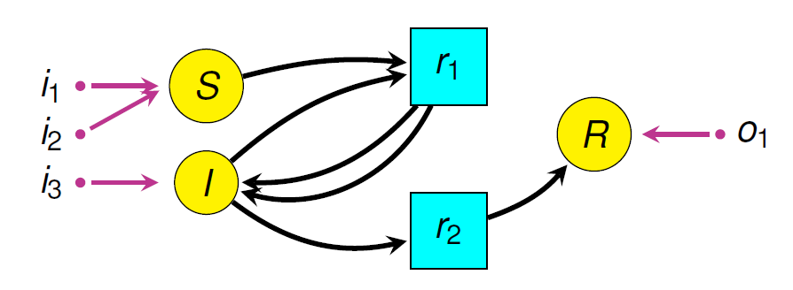
The picture here shows an example: a simple disease model where Susceptible people become Infective, then Recovered, then Susceptible again.

The boxes are “stocks” and the double-edged arrows are “flows”. There are also blue “links” from stocks to “variables”, and from stocks and variables to flows. This picture doesn’t show the formulas that say exactly how the variables depend on stocks, and how the flows depend on stocks and variables. So, this picture doesn’t show the whole thing. It’s really just what they call a “system structure diagram”: a stock-flow diagram missing the quantitative information that you need to get a system of ODEs from it. A stock-flow diagram, on the other hand, uniquely specifies a system of first-order ODEs.

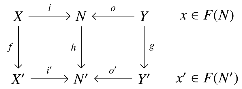
Modelers often regard diagrams as an informal step toward a mathematically rigorous formulation of a model in terms of ODEs. However, we’ve shown that stock-flow diagrams have a precise mathematical syntax! They are objects in a category while “open” stock-flow diagrams, where things can flow in and out of the whole system, are horizontal 1-cells in a double category If you know category theory you can read a paper we wrote with Evan Patterson where we explain this:

• John C. Baez, Xiaoyan Li, Sophie Libkind, Nathaniel D. Osgood and Evan Patterson, Compositional modeling with stock and flow diagrams. To appear in Proceedings of Applied Category Theory 2022.

If you don’t, we have a gentler paper for you:

• John C. Baez, Xiaoyan Li, Sophie Libkind, Nathaniel D. Osgood and Evan Redekopp, A categorical framework for modeling with stock and flow diagrams, to appear in Mathematics for Public Health, Springer, Berlin.

Why does it help to formalize the syntax of stock-flow diagrams using category theory? There are many reasons, but here are three:

1. Functorial Semantics

Our software lets modelers separate the syntax of stock and flow diagrams from their semantics: that is, the various uses to which these diagrams are put. Different choices of semantics are described via different functors. This idea, called “functorial semantics”, goes back to Lawvere and is popular in certain realms of theoretical computer science.

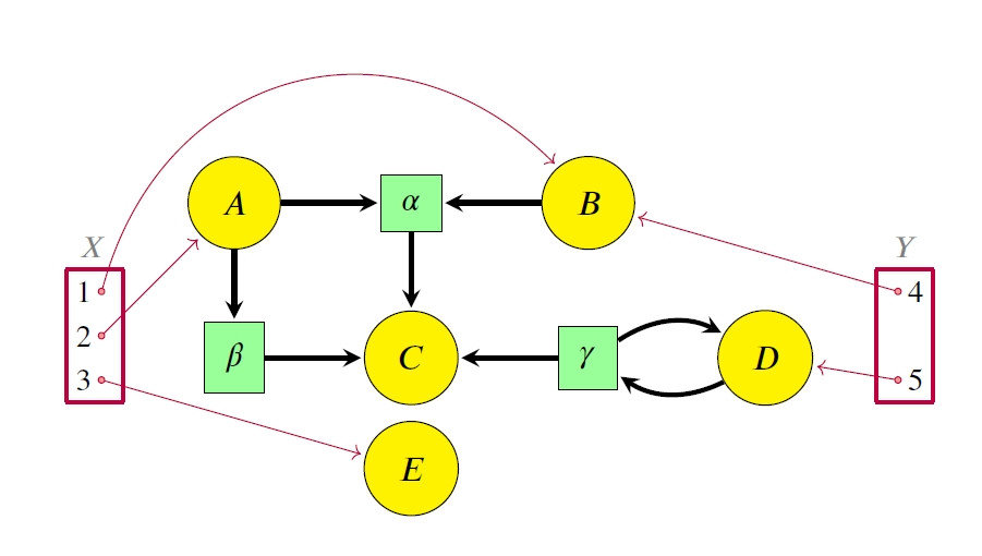
Besides the ODE semantics, we have implemented functors that turn stock-flow diagrams into other widely used diagrams: “system structure diagrams”, which I already explained, and “causal loop diagrams”. It doesn’t really matter much here, but a causal loop diagram ignores the distinction between stocks, flows and variables, lumps them all together, and has arrows saying what affects what:

These other forms of semantics capture purely qualitative features of stock and flow models. In the future, people can implement still more forms of semantics, like stochastic differential equation models!

So, instead of a single monolithic model, we have something much more flexible.

2. Composition

ModelCollab provides a structured way to build complex stock-flow diagrams from small reusable pieces. These pieces are open stock-flow diagrams, and sticking together amounts to composing them.

ModelCollab lets users save these diagrams and retrieve them for reuse as parts of various larger models. Since ModelCollab can run on multiple web browsers, it lets members of a modeling team compose models collaboratively. This is a big advance on current systems, which are not optimized for collaborative work.

This picture shows two small stock-flow diagrams being composed in ModelCollab:

Some of the underlying math here was developed in earlier work using categories and epidemiological modeling, which was also done by people at Topos and their collaborators:

• Sophie Libkind, Andrew Baas, Micah Halter, Evan Patterson and James P. Fairbanks, An algebraic framework for structured epidemic modelling, Philosophical Transactions of the Royal Society A 380 (2022), 20210309.

3. Stratification

Our software also allows users to “stratify” models: that is, refine them by subdividing a single population (stock) into several smaller populations with distinct features. For example, you might take a disease model and break each stock into different age groups.

In contrast to the global changes commonly required to stratify stock-flow diagrams, our software lets users build a stratified diagram as a “pullback” of simpler diagrams, which can be saved for reuse. Pullbacks are a concept from category theory, and here we are using pullbacks in the category whose objects are system structure diagrams. Remember, these are like stock and flow diagrams, but lacking the quantitative information describing the rates of flows. After a system structure diagram has been constructed, this information can be added to obtain a stock and flow diagram.

This picture shows two different models stratified in two different ways, creating four larger models. I won’t try to really explain this here. But at least you can get a tiny glimpse of how complicated these models get. They get a lot bigger! That’s why we need software based on good math to deal with them efficiently.

References

[AJ] AlgebraicJulia: Bringing compositionality to technical computing.

[B1] John C. Baez, Xiaoyan Li, Sophie Libkind, Nathaniel D. Osgood and Evan Patterson, Compositional modeling with stock and flow diagrams. To appear in Proceedings of Applied Category Theory 2022.

[B2] John C. Baez, Xiaoyan Li, Sophie Libkind, Nathaniel D. Osgood and Eric Redekopp, A categorical framework for modeling with stock and flow diagrams, to appear in Mathematics for Public Health, Springer, Berlin.

[H] P. S. Hovmand, Community Based System Dynamics, Springer, Berlin, 2014.

[L] Sophie Libkind, Andrew Baas, Micah Halter, Evan Patterson and James P. Fairbanks, An algebraic framework for structured epidemic modelling, Philosophical Transactions of the Royal Society A 380 (2022), 20210309.

[MC] ModelCollab: A web-based application for collaborating on simulation models in real-time using Firebase.

[SF] Stockflow.jl.

Symposium on Compositional Structures 9

The Symposium on Compositional Structures is a nice informal conference series that happens more than once a year. You can now submit talks for this one.

• Ninth Symposium on Compositional Structures (SYCO 9), Como, Italy, 8-9 September 2022. Deadline to submit a talk: Monday 1 August 2022.

Apparently you can attend online but to give a talk you have to go there. Here are some details:

The Symposium on Compositional Structures (SYCO) is an interdisciplinary series of meetings aiming to support the growing community of researchers interested in the phenomenon of compositionality, from both applied and abstract perspectives, and in particular where category theory serves as a unifying common language. Previous SYCO events have been held in Birmingham, Strathclyde, Oxford, Chapman, Leicester and Tallinn.

We welcome submissions from researchers across computer science, mathematics, physics, philosophy, and beyond, with the aim of fostering friendly discussion, disseminating new ideas, and spreading knowledge between fields. Submission is encouraged for both mature research and work in progress, and by both established academics and junior researchers, including students. Submissions is easy, with no formatting or page restrictions. The meeting does not have proceedings, so work can be submitted even if it has been submitted or published elsewhere. You could submit work-in-progress, or a recently completed paper, or even a PhD or Masters thesis.

While no list of topics could be exhaustive, SYCO welcomes submissions with a compositional focus related to any of the following areas, in particular from the perspective of category theory:

• logical methods in computer science, including classical and quantum programming, type theory, concurrency, natural language processing and machine learning;
• graphical calculi, including string diagrams, Petri nets and reaction networks;
• languages and frameworks, including process algebras, proof nets, type theory and game semantics;
• abstract algebra and pure category theory, including monoidal category theory, higher category theory, operads, polygraphs, and relationships to homotopy theory;
• quantum algebra, including quantum computation and representation theory;
• tools and techniques, including rewriting, formal proofs and proof assistants, and game theory;
• industrial applications, including case studies and real-world problem descriptions.

Important dates

All deadlines are 23:59 Anywhere on Earth.

Submission deadline: Monday 1 August
Author notification: Monday 8 August 2022
Symposium dates: Thursday 8 and Friday 9 September 2022

Submission instructions

Submissions are by EasyChair, via the SYCO 9 submission page:

• https://easychair.org/my/conference?conf=syco9

Submission is easy, with no format requirements or page restrictions. The meeting does not have proceedings, so work can be submitted even if it has been submitted or published elsewhere. Think creatively: you could submit a recent paper, or notes on work in progress, or even a recent Masters or PhD thesis.

In the event that more good-quality submissions are received than can be accommodated in the timetable, the programme committee may choose to defer some submissions to a future meeting, rather than reject them. Deferred submissions can be re-submitted to any future SYCO meeting, where they will not need peer review, and where they will be prioritised for inclusion in the programme. Meetings will be held sufficiently frequently to avoid a backlog of deferred papers.

If you have a submission which was deferred from a previous SYCO meeting, it will not automatically be considered for SYCO 9; you still need to submit it again through EasyChair. When submitting, append the words “DEFERRED FROM SYCO X” to the title of your paper, replacing “X” with the appropriate meeting number. There is no need to attach any documents.

Programme committee

The PC chair is John van de Wetering, Radboud University. The Programme Committee will be announced soon.

Steering committee

Ross Duncan, University of Strathclyde
Chris Heunen, University of Edinburgh
Dominic Horsman, University of Oxford
Aleks Kissinger, University of Oxford
Samuel Mimram, École Polytechnique
Simona Paoli, University of Aberdeen
Mehrnoosh Sadrzadeh, University College London
Pawel Sobocinski, Tallinn University of Technology
Jamie Vicary, University of Cambridge

Structured vs Decorated Cospans (Part 2)

Decorated cospans are a framework for studying open systems invented by Brendan Fong. Since I’m now visiting the institute he and David Spivak set up—the Topos Institute—it was a great time to give a talk explaining the history of decorated cospans, their problems, and how those problems have been solved:

Structured vs Decorated Cospans

Abstract. One goal of applied category theory is to understand open systems: that is, systems that can interact with the external world. We compare two approaches to describing open systems as morphisms: structured and decorated cospans. Each approach provides a symmetric monoidal double category. Structured cospans are easier, decorated cospans are more general, but under certain conditions the two approaches are equivalent. We take this opportunity to explain some tricky issues that have only recently been resolved.

It’s probably best to get the slides here and look at them while watching this video:

If you prefer a more elementary talk explaining what structured and decorated cospans are good for, try these slides.

For videos and slides of two related talks go here:

• Structured cospans and double categories.

• Structured cospans and Petri nets.

For more, read these:

• Brendan Fong, Decorated cospans.

• Evan Patterson and Micah Halter, Compositional epidemiological modeling using structured cospans.

• John Baez and Kenny Courser, Structured cospans.

• John Baez, Kenny Courser and Christina Vasilakopoluou, Structured versus decorated cospans.

• Kenny Courser, Open Systems: a Double Categorical Perspective.

• Michael Shulman, Framed bicategories and monoidal fibrations.

• Joe Moeller and Christina Vasilakopolou, Monoidal Grothendieck construction.

To read more about the network theory project, go here:

• Network Theory.

Complex Adaptive System Design (Part 10)

guest post by John Foley

Though the Complex Adaptive System Composition and Design Environment (CASCADE) program concluded in Fall 2020, just this week two new articles came out reviewing the work and future research directions:

• John Baez and John Foley, Operads for designing systems of systems, Notices of the American Mathematical Society 68 (2021), 1005–1007.

• John Foley, Spencer Breiner, Eswaran Subrahmanian and John Dusel, Operads for complex system design specification, analysis and synthesis, Proceedings of the Royal Society A 477 (2021), 20210099.

Operads for Designing Systems of Systems

The first is short and sweet (~2 pages!), aimed at a general mathematical audience. It describes the motivation for CASCADE and how basic modeling issues for point-to-point communications led to the development network operads:

This figure depicts the prototypical example of this style of operad, the ‘simple network operad’, acting on an algebra of graphs whose nodes are endowed with locations and edges can be no longer than a fixed range limit. For more information, check out the article or Part 4 of this series.

For a quick, retrospective overview of CASCADE, this note is hard to beat, so I won’t repeat more here.

Operads for complex system design specification, analysis and synthesis

The second article is a full length review, aimed at a general applied science audience:

We introduce operads for design to a general scientific audience by explaining what the operads do relative to broadly applied techniques and how specific domain problems are modelled. Research directions are presented with an eye towards opening up interdisciplinary partnerships and continuing application-driven investigations to build on recent insights.

The review describes how operads apply to system design problems through three examples:

and concludes with a discussion of future research directions. The specification and synthesis examples come from applications of network operads in CASCADE, but the analysis example was contributed by collaborators Spencer Breiner and Eswaran Subrahmanian at the National Institute of Standards and Technology (NIST), who analyzed the Length Scale Interferometer (LSI) at NIST headquarters. Readers interested in a quick introduction to these examples should head directly to Section 3 of the review.

As we describe:

The present article captures an intermediate stage of technical maturity: operad-based design has shown its practicality by lowering barriers of entry for applied practitioners and demonstrating applied examples across many domains. However, it has not realized its full potential as an applied meta-language. Much of this recent progress is not focused solely on the analytic power of operads to separate concerns. Significant progress on explicit specification of domain models and techniques to automatically synthesize designs from basic building blocks has been made.

With this context, CASCADE’s contribution was prototyping general-purpose methods to specify basic building blocks and synthesize composite systems from atoms. By testing these methods against specific domain problems, we learned that domain-specific information should be exploited but systematically fitting together general-purpose and computationally efficient methods is challenging. Moreover, no reconciliation between the analytic point-of-view on operads for system design and the `generative’ perspective of network operads, which facilitate specification and synthesis, has been established. The review does not address how these threads might fit together precisely, but perhaps the answer looks something like this:

For more discussion of future research directions, please see Section 7 of the review, especially the open problems listed in 7f.

For readers that make it through the examples in Sections 4, 5 and 6 of the review but still want more, the following references provide additional details:

• John Baez, John Foley, Joe Moeller and Blake Pollard, Network models, Theory and Applications of Categories 35 (2020), 700–744.

• Spencer Breiner, Olivier Marie-Rose, Blake Pollard and Eswaran Subrahmanian, Modeling hierarchical system with operads, Electron. Proc. Theor. Comput. Sci. 323 (2020) 72–83.

• John Baez, John Foley and Joe Moeller, Network models from Petri nets with catalysts, Compositionality 1 (4) (2017).

---

Here’s the whole series of posts:

• Part 1. CASCADE: the Complex Adaptive System Composition and Design Environment.

• Part 2. Metron’s software for system design.

• Part 3. Operads: the basic idea.

• Part 4. Network operads: an easy example.

• Part 5. Algebras of network operads: some easy examples.

• Part 6. Network models.

• Part 7. Step-by-step compositional design and tasking using commitment networks.

• Part 8. Compositional tasking using category-valued network models.

• Part 9 – Network models from Petri nets with catalysts.

• Part 10 – Two papers reviewing the whole project.

Symmetric Monoidal Categories: a Rosetta Stone

The Topos Institute is in business! I’m really excited about visiting there this summer and working on applied category theory.

They recently had a meeting with some people concerned about AI risks, called Finding the Right Abstractions, organized by Scott Garrabrant, David Spivak, and Andrew Critch. I gave a gentle introduction to the uses of symmetric monoidal categories:

• Symmetric monoidal categories: a Rosetta Stone.

To describe systems composed of interacting parts, scientists and engineers draw diagrams of networks: flow charts, Petri nets, electrical circuit diagrams, signal-flow graphs, chemical reaction networks, Feynman diagrams and the like. All these different diagrams fit into a common framework: the mathematics of symmetric monoidal categories. While originally the morphisms in such categories were mainly used to describe processes, we can also use them to describe open systems.

You can see the slides here, and watch a video here:

For a lot more detail on these ideas, see:

• John Baez and Mike Stay, Physics, topology, logic and computation: a Rosetta Stone, in New Structures for Physics, ed. Bob Coecke, Lecture Notes in Physics vol. 813, Springer, Berlin, 2011, pp. 95—174.

Non-Equilibrium Thermodynamics in Biology (Part 1)

Together with William Cannon and Larry Li, I’m helping run a minisymposium as part of SMB2021, the annual meeting of the Society for Mathematical Biology:

• Non-equilibrium Thermodynamics in Biology: from Chemical Reaction Networks to Natural Selection, Monday June 14, 2021, beginning 9:30 am Pacific Time.

You can register for free here before May 31st, 11:59 pm Pacific Time. You need to register to watch the talks live on Zoom. I think the talks will be recorded.

Here’s the idea:

Abstract: Since Lotka, physical scientists have argued that living things belong to a class of complex and orderly systems that exist not despite the second law of thermodynamics, but because of it. Life and evolution, through natural selection of dissipative structures, are based on non-equilibrium thermodynamics. The challenge is to develop an understanding of what the respective physical laws can tell us about flows of energy and matter in living systems, and about growth, death and selection. This session will address current challenges including understanding emergence, regulation and control across scales, and entropy production, from metabolism in microbes to evolving ecosystems.

It’s exciting to me because I want to get back into work on thermodynamics and reaction networks, and we’ll have some excellent speakers on these topics. I think the talks will be in this order… later I will learn the exact schedule.

Christof Mast, Ludwig-Maximilians-Universität München

Coauthors: T. Matreux, K. LeVay, A. Schmid, P. Aikkila, L. Belohlavek, Z. Caliskanoglu, E. Salibi, A. Kühnlein, C. Springsklee, B. Scheu, D. B. Dingwell, D. Braun, H. Mutschler.

Title: Heat flows adjust local ion concentrations in favor of prebiotic chemistry

Abstract: Prebiotic reactions often require certain initial concentrations of ions. For example, the activity of RNA enzymes requires a lot of divalent magnesium salt, whereas too much monovalent sodium salt leads to a reduction in enzyme function. However, it is known from leaching experiments that prebiotically relevant geomaterial such as basalt releases mainly a lot of sodium and only little magnesium. A natural solution to this problem is heat fluxes through thin rock fractures, through which magnesium is actively enriched and sodium is depleted by thermogravitational convection and thermophoresis. This process establishes suitable conditions for ribozyme function from a basaltic leach. It can take place in a spatially distributed system of rock cracks and is therefore particularly stable to natural fluctuations and disturbances.

Supriya Krishnamurthy, Stockholm University

Coauthors: Eric Smith

Title: Stochastic chemical reaction networks

Abstract: The study of chemical reaction networks (CRNs) is a very active field. Earlier well-known results (Feinberg Chem. Enc. Sci. 42 2229 (1987), Anderson et al Bull. Math. Biol. 72 1947 (2010)) identify a topological quantity called deficiency, easy to compute for CRNs of any size, which, when exactly equal to zero, leads to a unique factorized (non-equilibrium) steady-state for these networks. No general results exist however for the steady states of non-zero-deficiency networks. In recent work, we show how to write the full moment-hierarchy for any non-zero-deficiency CRN obeying mass-action kinetics, in terms of equations for the factorial moments. Using these, we can recursively predict values for lower moments from higher moments, reversing the procedure usually used to solve moment hierarchies. We show, for non-trivial examples, that in this manner we can predict any moment of interest, for CRNs with non-zero deficiency and non-factorizable steady states. It is however an open question how scalable these techniques are for large networks.

Pierre Gaspard, Université libre de Bruxelles

Title: Nonequilibrium biomolecular information processes

Abstract: Nearly 70 years have passed since the discovery of DNA structure and its role in coding genetic information. Yet, the kinetics and thermodynamics of genetic information processing in DNA replication, transcription, and translation remain poorly understood. These template-directed copolymerization processes are running away from equilibrium, being powered by extracellular energy sources. Recent advances show that their kinetic equations can be exactly solved in terms of so-called iterated function systems. Remarkably, iterated function systems can determine the effects of genome sequence on replication errors, up to a million times faster than kinetic Monte Carlo algorithms. With these new methods, fundamental links can be established between molecular information processing and the second law of thermodynamics, shedding a new light on genetic drift, mutations, and evolution.

Carsten Wiuf, University of Copenhagen

Coauthors: Elisenda Feliu, Sebastian Walcher, Meritxell Sáez

Title: Reduction and the Quasi-Steady State Approximation

Abstract: Chemical reactions often occur at different time-scales. In applications of chemical reaction network theory it is often desirable to reduce a reaction network to a smaller reaction network by elimination of fast species or fast reactions. There exist various techniques for doing so, e.g. the Quasi-Steady-State Approximation or the Rapid Equilibrium Approximation. However, these methods are not always mathematically justifiable. Here, a method is presented for which (so-called) non-interacting species are eliminated by means of QSSA. It is argued that this method is mathematically sound. Various examples are given (Michaelis-Menten mechanism, two-substrate mechanism, …) and older related techniques from the 50-60ies are briefly discussed.

Matteo Polettini, University of Luxembourg

Coauthor: Tobias Fishback

Title: Deficiency of chemical reaction networks and thermodynamics

Abstract: Deficiency is a topological property of a Chemical Reaction Network linked to important dynamical features, in particular of deterministic fixed points and of stochastic stationary states. Here we link it to thermodynamics: in particular we discuss the validity of a strong vs. weak zeroth law, the existence of time-reversed mass-action kinetics, and the possibility to formulate marginal fluctuation relations. Finally we illustrate some subtleties of the Python module we created for MCMC stochastic simulation of CRNs, soon to be made public.

Ken Dill, Stony Brook University

Title: The principle of maximum caliber of nonequilibria

Abstract: Maximum Caliber is a principle for inferring pathways and rate distributions of kinetic processes. The structure and foundations of MaxCal are much like those of Maximum Entropy for static distributions. We have explored how MaxCal may serve as a general variational principle for nonequilibrium statistical physics – giving well-known results, such as the Green-Kubo relations, Onsager’s reciprocal relations and Prigogine’s Minimum Entropy Production principle near equilibrium, but is also applicable far from equilibrium. I will also discuss some applications, such as finding reaction coordinates in molecular simulations non-linear dynamics in gene circuits, power-law-tail distributions in “social-physics” networks, and others.

Joseph Vallino, Marine Biological Laboratory, Woods Hole

Coauthors: Ioannis Tsakalakis, Julie A. Huber

Title: Using the maximum entropy production principle to understand and predict microbial biogeochemistry

Abstract: Natural microbial communities contain billions of individuals per liter and can exceed a trillion cells per liter in sediments, as well as harbor thousands of species in the same volume. The high species diversity contributes to extensive metabolic functional capabilities to extract chemical energy from the environment, such as methanogenesis, sulfate reduction, anaerobic photosynthesis, chemoautotrophy, and many others, most of which are only expressed by bacteria and archaea. Reductionist modeling of natural communities is problematic, as we lack knowledge on growth kinetics for most organisms and have even less understanding on the mechanisms governing predation, viral lysis, and predator avoidance in these systems. As a result, existing models that describe microbial communities contain dozens to hundreds of parameters, and state variables are extensively aggregated. Overall, the models are little more than non-linear parameter fitting exercises that have limited, to no, extrapolation potential, as there are few principles governing organization and function of complex self-assembling systems. Over the last decade, we have been developing a systems approach that models microbial communities as a distributed metabolic network that focuses on metabolic function rather than describing individuals or species. We use an optimization approach to determine which metabolic functions in the network should be up regulated versus those that should be down regulated based on the non-equilibrium thermodynamics principle of maximum entropy production (MEP). Derived from statistical mechanics, MEP proposes that steady state systems will likely organize to maximize free energy dissipation rate. We have extended this conjecture to apply to non-steady state systems and have proposed that living systems maximize entropy production integrated over time and space, while non-living systems maximize instantaneous entropy production. Our presentation will provide a brief overview of the theory and approach, as well as present several examples of applying MEP to describe the biogeochemistry of microbial systems in laboratory experiments and natural ecosystems.

Gheorge Craciun, University of Wisconsin-Madison

Title: Persistence, permanence, and global stability in reaction network models: some results inspired by thermodynamic principles

Abstract: The standard mathematical model for the dynamics of concentrations in biochemical networks is called mass-action kinetics. We describe mass-action kinetics and discuss the connection between special classes of mass-action systems (such as detailed balanced and complex balanced systems) and the Boltzmann equation. We also discuss the connection between the “global attractor conjecture” for complex balanced mass-action systems and Boltzmann’s H-theorem. We also describe some implications for biochemical mechanisms that implement noise filtering and cellular homeostasis.

Hong Qian, University of Washington

Title: Large deviations theory and emergent landscapes in biological dynamics

Abstract: The mathematical theory of large deviations provides a nonequilibrium thermodynamic description of complex biological systems that consist of heterogeneous individuals. In terms of the notions of stochastic elementary reactions and pure kinetic species, the continuous-time, integer-valued Markov process dictates a thermodynamic structure that generalizes (i) Gibbs’ macroscopic chemical thermodynamics of equilibrium matters to nonequilibrium small systems such as living cells and tissues; and (ii) Gibbs’ potential function to the landscapes for biological dynamics, such as that of C. H. Waddington’s and S. Wright’s.

John Harte, University of Berkeley

Coauthors: Micah Brush, Kaito Umemura

Title: Nonequilibrium dynamics of disturbed ecosystems

Abstract: The Maximum Entropy Theory of Ecology (METE) predicts the shapes of macroecological metrics in relatively static ecosystems, across spatial scales, taxonomic categories, and habitats, using constraints imposed by static state variables. In disturbed ecosystems, however, with time-varying state variables, its predictions often fail. We extend macroecological theory from static to dynamic, by combining the MaxEnt inference procedure with explicit mechanisms governing disturbance. In the static limit, the resulting theory, DynaMETE, reduces to METE but also predicts a new scaling relationship among static state variables. Under disturbances, expressed as shifts in demographic, ontogenic growth, or migration rates, DynaMETE predicts the time trajectories of the state variables as well as the time-varying shapes of macroecological metrics such as the species abundance distribution and the distribution of metabolic rates over individuals. An iterative procedure for solving the dynamic theory is presented. Characteristic signatures of the deviation from static predictions of macroecological patterns are shown to result from different kinds of disturbance. By combining MaxEnt inference with explicit dynamical mechanisms of disturbance, DynaMETE is a candidate theory of macroecology for ecosystems responding to anthropogenic or natural disturbances.

Structured vs Decorated Cospans (Part 1)

Some of us just finished a paper clarifying the connection between two approaches to describing open systems—that is, systems that can interact with their environment, and can be composed to form larger open systems:

• John Baez, Kenny Courser and Christina Vasilakopolou, Structured versus decorated cospans.

And, next week I’m giving a talk about it at YAMCaTS! This is not a conference for felines who like sweet potatoes: it’s the Yorkshire and Midlands Category Seminar, organized by Simona Paoli, Nicola Gambino and Steve Vickers.

In my talk, I’ll start by sketching some ideas behind Halter and Patterson’s software for quickly assembling larger models of COVID-19 from smaller models. Then, I’ll dig deeper into the underlying math, where we use ‘structured’ or ‘decorated’ cospans to model open systems.

This quickly gets into some serious category theory—and since YAMCaTS is a category theory seminar, I won’t shy away from that. Here are my slides:

• John Baez, Structured vs decorated cospans, YAMCaTS, Friday 5 February 2021, 17:00 UTC. Zoom link here, meeting ID 810 4239 7132; to get in use 68302x where x is a one-digit perfect number.

Abstract. One goal of applied category theory is to understand open systems: that is, systems that can interact with the external world. We compare two approaches to describing open systems as cospans equipped with extra data: structured and decorated cospans. Each approach provides a symmetric monoidal double category, and we prove that under certain conditions these symmetric monoidal double categories are isomorphic. We illustrate these ideas with applications to dynamical systems and epidemiological modeling. This is joint work with Kenny Courser and Christina Vasilakopoulou.

I don’t know if my talk will be recorded, but it will be on Zoom so recording it would be easy, and I’ll try to get the organizers to do that.

For videos and slides of two related talks go here:

• Structured cospans and double categories.

• Structured cospans and Petri nets.

For more, read these:

• Evan Patterson and Micah Halter, Compositional epidemiological modeling using structured cospans.

• John Baez and Kenny Courser, Structured cospans.

• Kenny Courser, Open Systems: a Double Categorical Perspective. (Blog articles here.)

• Michael Shulman, Framed bicategories and monoidal fibrations.

• Joe Moeller and Christina Vasilakopolou, Monoidal Grothendieck construction.

To read more about the network theory project, go here:

• Network theory.

Open Systems: A Double Categorical Perspective (Part 3)

Back to Kenny Courser’s thesis:

• Kenny Courser, Open Systems: A Double Categorical Perspective, Ph.D. thesis, U. C. Riverside, 2020.

Last time I explained the problems with decorated cospans as a framework for dealing with open systems. I vaguely hinted that Kenny’s thesis presents two solutions to these problems: so-called ‘structured cospans’, and a new improved approach to decorated cospans. Now let me explain these!

You may wonder why I’m returning to this now, after three months of silence. The reason is that Kenny, Christina Vasilakopolou, and I just finished a paper that continues this story:

• John Baez, Kenny Courser and Christina Vasilakopoulou, Structured versus decorated cospans.

We showed that under certain conditions, structured and decorated cospans are equivalent. So, I’m excited about this stuff again.

Last time I explained Fong’s theorem about decorated cospans:

Fong’s Theorem. Suppose is a category with finite colimits, and make into a symmetric monoidal category with its coproduct as the tensor product. Suppose is a symmetric lax monoidal functor. Define an F-decorated cospan to be a cospan

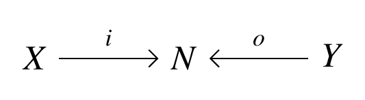
in together with an element called a decoration. Then there is a symmetric monoidal category with

• objects of as objects,
• isomorphism classes of -decorated cospans as morphisms.

The theorem is true, but it doesn’t apply to all the examples we wanted it to. The problem is that it’s ‘not categorified enough’. It’s fine if we want to decorate the apex of our cospan with some extra structure: we do this by choosing an element of some set But in practice, we often want to decorate with some extra stuff, which means choosing an object of a category So we should really use not a functor

but something like a functor

What do I mean by ‘something like a functor?’ Well, is not just a category but a 2-category: it has categories as objects, functors as morphisms, but also natural transformations as 2-morphisms. The natural notion of ‘something like a functor’ from a category to a 2-category is called a pseudofunctor. And just as we can define symmetric lax monoidal functor, we can define a symmetric lax monoidal pseudofunctor.

All these nuances really matter when we’re studying open graphs, as we were last time!

Here we want the feet of our structured cospan to be finite sets and the apex to be a finite graph. So, we have and for any we want to be the set, or category, of finite graphs having as their set of nodes.

I explained last time all the disasters that ensue when you try to let be the set of finite graphs having as its set of nodes. You can try, but you will pay dearly for it! You can struggle and fight, like Hercules trying to chop all the heads off the Hydra, but you still can’t get a symmetric lax monoidal functor

that sends any finite set to the set of graphs having as their set of nodes.

But there is a perfectly nice category of all finite graphs having as their set of nodes. And you can get a symmetric lax monoidal pseudofunctor

that sends any any finite set to the category of finite graphs having it as nodes. So you should stop fighting and go with the flow.

Kenny, Christina and I proved an enhanced version of Fong’s theorem that works starting from this more general kind of And instead of just giving you a symmetric monoidal category, this theorem gives you a symmetric monoidal double category.

In fact, that is something you should have wanted already, even with Fong’s original hypotheses! The clue is that Fong’s theorem uses isomorphism classes of decorated cospans, which suggests we’d get something better if we used decorated cospans themselves. Kenny tackled this a while ago, getting a version of Fong’s theorem that produces a symmetric monoidal double category, and another version that produces a symmetric monoidal bicategory:

• Kenny Courser, A bicategory of decorated cospans, Theory and Applications of Categories 32 (2017), 995–1027.

Over the years we’ve realized that the double category is better, because it contains more information and is easier to work with. So, in our new improved approach to decorated cospans, we go straight for the jugular and get a double category. And here’s how it works:

Theorem. Suppose is a category with finite colimits, and make into a symmetric monoidal category with its coproduct as the tensor product. Suppose is a symmetric lax monoidal pseudofunctor. Then there is a symmetric monoidal double category in which

• an object is an object of
• a vertical morphism is a morphism in
• a horizontal morphism is an F-decorated cospan, meaning a cospan in together with a decoration:

• a 2-morphism is a map of decorated cospans, meaning a commutative diagram in :

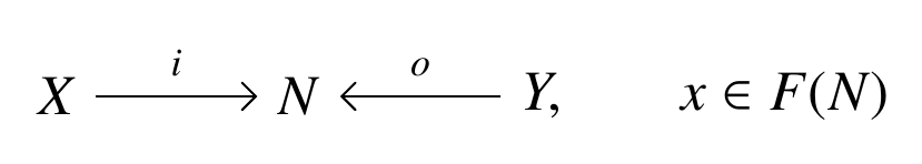
together with a morphism the map of decorations.

We call a decorated cospan double category. And as our paper explains, this idea lets us fix all the broken attempted applications of Fong’s original decorated cospan categories!

All this is just what any category theorist worth their salt would try, in order to fix the original problems with decorated cospans. It turns out that proving the theorem above is not so easy, mainly because the definition of ‘symmetric monoidal double category’ is rather complex. But if you accept the theorem—including the details of how you get the symmetric monoidal structure on the double category, which I have spared you here—then it doesn’t really matter much that the proof takes work.

Next time I’ll tell you about the other way to fix the original decorated cospan formalism: structured cospans. When these work, they are often easier to use.

---

• Part 1: an overview of Courser’s thesis and related papers.

• Part 2: problems with the original decorated cospans.

• Part 3: the new improved decorated cospans.

Categories of Nets (Part 2)

guest post by Michael Shulman

Now that John gave an overview of the Petri nets paper that he and I have just written with Jade and Fabrizio, I want to dive a bit more into what we accomplish. The genesis of this paper was a paper written by Fabrizio and several other folks entitled Computational Petri Nets: Adjunctions Considered Harmful, which of course sounds to a category theorist like a challenge. Our paper, and particularly the notion of Σ-net and the adjunction in the middle column relating Σ-nets to symmetric strict monoidal categories, is an answer to that challenge.

Suppose you wanted to “freely” generate a symmetric monoidal category from some combinatorial data. What could that data be? In other words (for a category theorist at least), what sort of category appears in an adjunction ? (By the way, all monoidal categories in this post will be strict, so I’m going to drop that adjective for conciseness.)

Perhaps the simplest choice is the same data that naturally generates a plain category, namely a directed graph. However, this is pretty limited in terms of what symmetric monoidal categories it can generate, since the generating morphisms will always only have single generating objects as their domain and codomain.

Another natural choice is the same data that naturally generates a multicategory, which might be called a “multigraph”: a set of objects together with, for every tuple of objects and single object , a set of arrows from to . In the generated symmetric monoidal category, such an arrow gives rise to a morphism ; thus we can now have multiple generating objects in the domains of generating morphisms, but not the codomains.

Of course, this suggests an even better solution: a set of objects, together with a set of arrows for every pair of tuples and . I’d be tempted to call this a “polygraph”, since it also naturally generates a polycategory. But other folks got there first and called it a “tensor scheme” and also a “pre-net”. In the latter case, the objects are called “places” and the morphisms “transitions”. But whatever we call it, it allows us to generate free symmetric monoidal categories in which the domains and codomains of generating morphisms can both be arbitrary tensor products of generating objects. For those who like fancy higher-categorical machinery, it’s the notion of computad obtained from the monad for symmetric monoidal categories.

However, pre-nets are not without flaws. One of the most glaring, for people who actually want to compute with freely generated symmetric monoidal categories, is that there aren’t enough morphisms between them. For instance, suppose one pre-net has three places and a transition , while a second pre-net has three places and a transition . Once we generate a symmetric monoidal category, then can be composed with a symmetry and similarly for ; so the symmetric monoidal categories generated by and are isomorphic. But there isn’t even a single map of pre-nets from to or vice versa, because a map of pre-nets has to preserve the ordering on the inputs and outputs. This is weird and annoying for combinatorial data that’s supposed to present a symmetric monoidal category.

Another way of making essentially the same point is that just as the adjunction between SMCs and directed graphs factors through categories, and the adjunction between SMCs and multigraphs factors through multicategories, the adjunction between SMCs and pre-nets factors through non-symmetric monoidal categories. In other words, a pre-net is really better viewed as data for generating a non-symmetric monoidal category, which we can then freely add symmetries to.

By contrast, in the objects that we call “Petri nets”, the domain and codomain of each generating morphism are elements of the free commutative monoid on the set of places—as opposed to elements of the free monoid, which is what they are for a pre-net. Thus, the domain of and above would be and respectively, which in a commutative monoid are equal (both are ). So the corresponding Petri nets of and are indeed isomorphic. However, once we squash everything down in this way, we lose the ability to functorially generate a symmetric monoidal category; all we can generate is a commutative monoidal category where all the symmetries are identities.

At this point we’ve described the upper row and the left- and right-hand columns in John’s diagram:

What’s missing is a kind of net in the middle that corresponds to symmetric monoidal categories. To motivate the definition of Σ-net, consider how to solve the problem above of the “missing morphisms”. We want to send to a “permuted version” of . For this to be implemented by an actual set-map, we need this “permuted version” to be present in the data of somehow. This suggests that the transitions should come with a permutation action like that of, say, a symmetric multicategory. 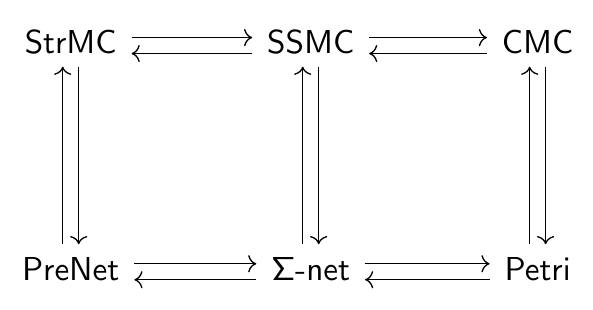Then inside we can actually act on by the transposition , yielding a new morphism which we can take to be the image of . Of course, we can also act on by other permutations, and likewise on ; but since these permutation actions are part of the structure they must be preserved by the morphism, so sending to uniquely determines where we have to send all these permutation images.

Now you can go back and look again at John’s definition of Σ-net: a set , a groupoid , and a discrete opfibration , where denotes the free-symmetric-strict-monoidal-category functor . Such a discrete opfibration is the same as a functor , and the objects of are the finite sequences of elements of while its morphisms are permutations; thus this is precisely a pre-net (the action of the functor on objects) with permutation actions as described above. I won’t get into the details of constructing the adjunction relating Σ-nets to symmetric monoidal categories; you can read the paper, or maybe I’ll blog about it later.

However, in solving the “missing morphisms” problem, we’ve introduced a new possibility. Suppose we act on by the transposition that switches the first two entries. We get another transition with the same domain and codomain as ; so it might equal , or it might not! In other words, transitions in a Σ-net can have isotropy. If , then when we generate a free symmetric monoidal category from our Σ-net, the corresponding morphism will have the property that when we compose it with the symmetry morphism we get back again. No symmetric monoidal category generated by a pre-net has this property; it’s more like the behavior of the commutative monoidal category generated by a Petri net, except that in the latter case the symmetry itself is the identity, rather than just acting by the identity on .

This suggests that Σ-nets can either “behave like pre-nets” or “behave like Petri nets”. This is made precise by the bottom row of adjunctions in the diagram. On one hand, we can map a pre-net to a Σ-net by freely generating the action of all permutations. This has a right adjoint that just forgets the permutation action (which actually has a further right adjoint, although that’s a bit weird). On the other hand, we can map a Petri net to a Σ-net by making all the permutations act as trivially as possible; this has a left adjoint that identifies each transition with all its permutation images. And these adjunctions commute with the three “free monoidal category” adjunctions in reasonable ways (see the paper for details).

The right adjoint mapping Petri nets into Σ-nets is fully faithful, so we really can say that Σ-nets “include” Petri nets. The left adjoint mapping pre-nets to Σ-nets is not fully faithful—it can’t possibly be, since the whole point of introducing Σ-nets was that pre-nets don’t have enough morphisms! But the full image of this functor is equivalent to a fourth kind of net: Kock’s whole-grain Petri nets. Kock’s approach to solving the problem of pre-nets is somewhat different, more analogous to the notion of “fat” symmetric monoidal category: he takes the domain and codomain of each transition to be a family of places indexed by a finite set. But his category turns out to be equivalent to the category of Σ-nets that are freely generated by some pre-net. (Kock actually proved this himself, as well as sketching the adjunction between Σ-nets and symmetric monoidal categories. He called Σ-nets “digraphical species”.)

So Σ-nets “include” both Petri nets and pre-nets, in an appropriate sense. The pre-nets (or, more precisely, whole-grain nets) are the Σ-nets with free permutation actions (trivial isotropy), while the Petri nets are the Σ-nets with trivial permutation actions (maximal isotropy). In Petri-net-ese, these correspond to the “individual token philosophy” and the “collective token philosophy”, respectively. (This makes it tempting to refer to the functors from Σ-nets to pre-nets and Petri nets as individuation and collectivization respectively.) But Σ-nets also allow us to mix and match the two philosophies, having some transitions with trivial isotropy, others with maximal isotropy, and still others with intermediate isotropy.

I like to think of Σ-nets as a Petri net analogue of orbifolds. Commutative-monoid-based Petri nets are like “coarse moduli spaces”, where we’ve quotiented by all symmetries but destroyed all the isotropy information; while whole-grain Petri nets are like manifolds, where we have no singularities but can only quotient by free actions. Pre-nets can then be thought of a “presentation” of a manifold, such as by a particular way of gluing coordinate patches together: useful in concrete examples, but not the “invariant” object we really want to study mathematically.

---

• Part 1: three kinds of nets, and the kinds of monoidal categories they generate.

• Part 2: what kind of net is best for generating symmetric monoidal categories?