Petri Net Programming (Part 2)

guest post by David A. Tanzer

An introduction to stochastic Petri nets

In the previous article, I explored a simple computational model called Petri nets. They are used to model reaction networks, and have applications in a wide variety of fields, including population ecology, gene regulatory networks, and chemical reaction networks. I presented a simulator program for Petri nets, but it had an important limitation: the model and the simulator contain no notion of the rates of the reactions. But these rates critically determine the character of the dynamics of network.

Here I will introduce the topic of ‘stochastic Petri nets,’ which extends the basic model to include reaction dynamics. Stochastic means random, and it is presumed that there is an underlying random process that drives the reaction events. This topic is rich in both its mathematical foundations and its practical applications. A direct application of the theory yields the rate equation for chemical reactions, which is a cornerstone of chemical reaction theory. The theory also gives algorithms for analyzing and simulating Petri nets.

We are now entering the ‘business’ of software development for applications to science. The business logic here is nothing but math and science itself. Our study of this logic is not an academic exercise that is tangential to the implementation effort. Rather, it is the first phase of a complete software development process for scientific programming applications.

The end goals of this series are to develop working code to analyze and simulate Petri nets, and to apply these tools to informative case studies. But we have some work to do en route, because we need to truly understand the models in order to properly interpret the algorithms. The key questions here are when, why, and to what extent the algorithms give results that are empirically predictive. We will therefore be embarking on some exploratory adventures into the relevant theoretical foundations.

The overarching subject area to which stochastic Petri nets belong has been described as stochastic mechanics in the network theory series here on Azimuth. The theme development here will partly parallel that of the network theory series, but with a different focus, since I am addressing a computationally oriented reader. For an excellent text on the foundations and applications of stochastic mechanics, see:

• Darren Wilkinson, Stochastic Modelling for Systems Biology, Chapman and Hall/CRC Press, Boca Raton, Florida, 2011.

Review of basic Petri nets

A Petri net is a graph with two kinds of nodes: species and transitions. The net is populated with a collection of ‘tokens’ that represent individual entities. Each token is attached to one of the species nodes, and this attachment indicates the type of the token. We may therefore view a species node as a container that holds all of the tokens of a given type.

The transitions represent conversion reactions between the tokens. Each transition is ‘wired’ to a collection of input species-containers, and to a collection of output containers. When it ‘fires’, it removes one token from each input container, and deposits one token to each output container.

Here is the example we gave, for a simplistic model of the formation and dissociation of H₂O molecules:

The circles are for species, and the boxes are for transitions.

The transition combine takes in two H tokens and one O token, and outputs one H₂O token. The reverse transition is split, which takes in one H₂O, and outputs two H’s and one O.

An important application of Petri nets is to the modeling of biochemical reaction networks, which include the gene regulatory networks. Since genes and enzymes are molecules, and their binding interactions are chemical reactions, the Petri net model is directly applicable. For example, consider a transition that inputs one gene G, one enzyme E, and outputs the molecular form G • E in which E is bound to a particular site on G.

Applications of Petri nets may differ widely in terms of the population sizes involved in the model. In general chemistry reactions, the populations are measured in units of moles (where a mole is ‘Avogadro’s number’ 6.022 · 10²³ entities). In gene regulatory networks, on the other hand, there may only be a handful of genes and enzymes involved in a reaction.

This difference in scale leads to a qualitative difference in the modelling. With small population sizes, the stochastic effects will predominate, but with large populations, a continuous, deterministic, average-based approximation can be used.

Representing Petri nets by reaction formulas

Petri nets can also be represented by formulas used for chemical reaction networks. Here is the formula for the Petri net shown above:

H₂O ↔ H + H + O

or the more compact:

H₂O ↔ 2 H + O

The double arrow is a compact designation for two separate reactions, which happen to be opposites of each other.

By the way, this reaction is not physically realistic, because one doesn’t find isolated H and O atoms traveling around and meeting up to form water molecules. This is the actual reaction pair that predominates in water:

2 H₂O ↔ OH^– + H₃O⁺

Here, a hydrogen nucleus H⁺, with one unit of positive charge, gets removed from one of the H₂O molecules, leaving behind the hydroxide ion OH^–. In the same stroke, this H⁺ gets re-attached to the other H₂O molecule, which thereby becomes a hydronium ion, H₃O⁺.

For a more detailed example, consider this reaction chain, which is of concern to the ocean environment:

CO₂ + H₂O ↔ H₂CO₃ ↔ H⁺ + HCO₃^–

This shows the formation of carbonic acid, namely H₂CO₃, from water and carbon dioxide. The next reaction represents the splitting of carbonic acid into a hydrogen ion and a negatively charged bicarbonate ion, HCO₃^–. There is a further reaction, in which a bicarbonate ion further ionizes into an H⁺ and a doubly negative carbonate ion CO₃^2-. As the diagram indicates, for each of these reactions, a reverse reaction is also present. For a more detailed description of this reaction network, see:

• Stephen E. Bialkowski, Carbon dioxide and carbonic acid.

Increased levels of CO₂ in the atmosphere will change the balance of these reactions, leading to a higher concentration of hydrogen ions in the water, i.e., a more acidic ocean. This is of concern because the metabolic processes of aquatic organisms is sensitive to the pH level of the water. The ultimate concern is that entire food chains could be disrupted, if some of the organisms cannot survive in a higher pH environment. See the Wikipedia page on ocean acidification for more information.

Exercise. Draw Petri net diagrams for these reaction networks.

Motivation for the study of Petri net dynamics

The relative rates of the various reactions in a network critically determine the qualitative dynamics of the network as a whole. This is because the reactions are ‘competing’ with each other, and so their relative rates determine the direction in which the state of the system is changing. For instance, if molecules are breaking down faster then they are being formed, then the system is moving towards full dissociation. When the rates are equal, the processes balance out, and the system is in an equilibrium state. Then, there are only temporary fluctuations around the equilibrium conditions.

The rate of the reactions will depend on the number of tokens present in the system. For example, if any of the input tokens are zero, then the transition can’t fire, and so its rate must be zero. More generally, when there are few input tokens available, there will be fewer reaction events, and so the firing rates will be lower.

Given a specification for the rates in a reaction network, we can then pose the following kinds of questions about its dynamics:

• Does the network have an equilibrium state?

• If so, what are the concentrations of the species at equilibrium?

• How quickly does it approach the equilibrium?

• At the equilibrium state, there will still be temporary fluctuations around the equilibrium concentrations. What are the variances of these fluctuations?

• Are there modes in which the network will oscillate between states?

This is the grail we seek.

Aside from actually performing empirical experiments, such questions can be addressed either analytically or through simulation methods. In either case, our first step is to define a theoretical model for the dynamics of a Petri net.

Stochastic Petri nets

A stochastic Petri net (with kinetics) is a Petri net that is augmented with a specification for the reaction dynamics. It is defined by the following:

• An underlying Petri net, which consists of species, transitions, an input map, and an output map. These maps assign to each transition a multiset of species. (Multiset means that duplicates are allowed.) Recall that the state of the net is defined by a marking function, that maps each species to its population count.

• A rate constant that is associated with each transition.

• A kinetic model, that gives the expected firing rate for each transition as a function of the current marking. Normally, this kinetic function will include the rate constant as a multiplicative factor.

A further ‘sanity constraint’ can be put on the kinetic function for a transition: it should give a positive value if and only if all of its inputs are positive.

• A stochastic model, which defines the probability distribution of the time intervals between firing events. This specific distribution of the firing intervals for a transition will be a function of the expected firing rate in the current marking.

This definition is based on the standard treatments found, for example in:

• M. Ajmone Marsan, Stochastic Petri nets: an elementary introduction, in Advances in Petri Nets, Springer, Berlin, 1989, 1–23.

or Wilkinson’s book mentioned above. I have also added an explicit mention of the kinetic model, based on the ‘kinetics’ described in here:

• Martin Feinberg, Lectures on chemical reaction networks.

There is an implied random process that drives the reaction events. A classical random process is given by a container with ‘particles’ that are randomly traveling around, bouncing off the walls, and colliding with each other. This is the general idea behind Brownian motion. It is called a random process because the outcome results from an ‘experiment’ that is not fully determined by the input specification. In this experiment, you pour in the ingredients (particles of different types), set the temperature (the distributions of the velocities), give it a stir, and then see what happens. The outcome consists of the paths taken by each of the particles.

In an important limiting case, the stochastic behavior becomes deterministic, and the population sizes become continuous. To see this, consider a graph of population sizes over time. With larger population sizes, the relative jumps caused by the firing of individual transitions become smaller, and graphs look more like continuous curves. In the limit, we obtain an approximation for high population counts, in which the graphs are continuous curves, and the concentrations are treated as continuous magnitudes. In a similar way, a pitcher of sugar can be approximately viewed as a continuous fluid.

This simplification permits the application of continuous mathematics to study of reaction network processes. It leads to the basic rate equation for reaction networks, which specifies the direction of change of the system as a function of the current state of the system.

In this article we will be exploring this continuous deterministic formulation of Petri nets, under what is known as the mass action kinetics. This kinetics is one implementation of the general specification of a kinetic model, as defined above. This means that it will define the expected firing rate of each transition, in a given marking of the net. The probabilistic variations in the spacing of the reactions—around the mean given by the expected firing rate—is part of the stochastic dynamics, and will be addressed in a subsequent article.

The mass-action kinetics

Under the mass action kinetics, the expected firing rate of a transition is proportional to the product of the concentrations of its input species. For instance, if the reaction were A + C → D, then the firing rate would be proportional to the concentration of A times the concentration of C, and if the reaction were A + A → D, it would be proportional to the square of the concentration of A.

This principle is explained by Feinberg as follows:

For the reaction A+C → D, an occurrence requires that a molecule of A meet a molecule of C in the reaction, and we take the probability of such an encounter to be proportional to the product [of the concentrations of A and C]. Although we do not presume that every such encounter yields a molecule of D, we nevertheless take the occurrence rate of A+C → D to be governed by [the product of the concentrations].

For an in-depth proof of the mass action law, see this article:

• Daniel Gillespie, A rigorous definition of the chemical master equation, 1992.

Note that we can easily pass back and forth between speaking of the population counts for the species, and the concentrations of the species, which is just the population count divided by the total volume V of the system. The mass action law applies to both cases, the only difference being that the constant factors of (1/V) used for concentrations will get absorbed into the rate constants.

The mass action kinetics is a basic law of empirical chemistry. But there are limits to its validity. First, as indicated in the proof in the Gillespie, the mass action law rests on the assumptions that the system is well-stirred and in thermal equilibrium. Further limits are discussed here:

• Georg Job and Regina Ruffler, Physical Chemistry (first five chapters), Section 5.2, 2010.

They write:

…precise measurements show that the relation above is not strictly adhered to. At higher concentrations, values depart quite noticeably from this relation. If we gradually move to lower concentrations, the differences become smaller. The equation here expresses a so-called “limiting law“ which strictly applies only when c → 0.

In practice, this relation serves as a useful approximation up to rather high concentrations. In the case of electrically neutral substances, deviations are only noticeable above 100 mol m⁻³. For ions, deviations become observable above 1 mol m⁻³, but they are so small that they are easily neglected if accuracy is not of prime concern.

Why would the mass action kinetics break down at high concentrations? According to the book quoted, it is due to “molecular and ionic interactions.” I haven’t yet found a more detailed explanation, but here is my supposition about what is meant by molecular interactions in this context. Doubling the number of A molecules doubles the number of expected collisions between A and C molecules, but it also reduces the probability that any given A and C molecules that are within reacting distance will actually react. The reaction probability is reduced because the A molecules are ‘competing’ for reactions with the C molecules. With more A molecules, it becomes more likely that a C molecule will simultaneously be within reacting distance of several A molecules; each of these A molecules reduces the probability that the other A molecules will react with the C molecule. This is most pronounced when the concentrations in a gas get high enough that the molecules start to pack together to form a liquid.

The equilibrium relation for a pair of opposite reactions

Suppose we have two opposite reactions:

Since the reactions have exactly opposite effects on the population sizes, in order for the population sizes to be in a stable equilibrium, the expected firing rates of and must be equal:

By mass action kinetics:

where means the concentration of

Hence at equilibrium:

So:

where is the equilibrium constant for the reaction pair.

Equilibrium solution for the formation and dissociation of a diatomic molecule

Let A be some type of atom, and let D = A₂ be the diatomic form of A. Then consider the opposite reactions:

From the preceding analysis, at equilibrium the following relation holds:

Let and be the population counts for A and B, and let

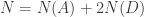
be the total number of units of A in the system, whether they be in the form of atoms or diatoms.

The value of is an invariant property of the system. The reactions cannot change it, because they are just shuffling the units of A from one arrangement to the other. By way of contrast, is not an invariant quantity.

Dividing this equation by the total volume , we get:

where is the concentration of the units of A.

Given a fixed value for and the rate constants and , we can then solve for the concentrations at equilibrium:

Since can’t be negative, only the positive square root is valid.

Here is the solution for the case where :

Conclusion

We’ve covered a lot of ground, starting with the introduction of the stochastic Petri net model, followed by a general discussion of reaction network dynamics, the mass action laws, and calculating equilibrium solutions for simple reaction networks.

We still have a number of topics to cover on our journey into the foundations, before being able to write informed programs to solve problems with stochastic Petri nets. Upcoming topics are (1) the deterministic rate equation for general reaction networks and its application to finding equilibrium solutions, and (2) an exploration of the stochastic dynamics of a Petri net. These are the themes that will support our upcoming software development.