Glyolysis is a way that organisms can get free energy from glucose without needing oxygen. Animals like you and me can do glycolysis, but we get more free energy from oxidizing glucose. Other organisms are anaerobic: they don’t need oxygen. And some, like yeast, survive mainly by doing glycolysis!
If you put yeast cells in water containing a constant low concentration of glucose, they convert it into alcohol at a constant rate. But if you increase the concentration of glucose something funny happens. The alcohol output starts to oscillate!
It’s not that the yeast is doing something clever and complicated. If you break down the yeast cells, killing them, this effect still happens. People think these oscillations are inherent to the chemical reactions in glycolysis.
I learned this after writing Part 1, thanks to Alan Rendall. I first met Alan when we were both working on quantum gravity. But last summer I met him in Copenhagen, where we both attending the workshop Trends in reaction network theory. It turned out that now he’s deep into the mathematics of biochemistry, especially chemical oscillations! He has a blog, and he’s written some great articles on glycolysis:
• Alan Rendall, Albert Goldbeter and glycolytic oscillations, Hydrobates, 21 January 2012.
• Alan Rendall, The Higgins–Selkov oscillator, Hydrobates, 14 May 2014.
In case you’re wondering, Hydrobates is the name of a kind of sea bird, the storm petrel. Alan is fond of sea birds. Since the ultimate goal of my work is to help our relationship with nature, this post is dedicated to the storm petrel:

The basics
Last time I gave a summary description of glycolysis:
2 pyruvate + 2 NADH + 2 H+ + 2 ATP + 2 H2O
The idea is that a single molecule of glucose:

gets split into two molecules of pyruvate:

The free energy released from this process is used to take two molecules of adenosine diphosphate or ADP:

and attach to each one phosphate group, typically found as phosphoric acid:

thus producing two molecules of adenosine triphosphate or ATP:

along with 2 molecules of water.
But in the process, something else happens too! 2 molecules of nicotinamide adenine dinucleotide NAD get reduced. That is, they change from the oxidized form called NAD+:

to the reduced form called NADH, along with two protons: that is, 2 H+.
Puzzle 1. Why does NAD+ have a little plus sign on it, despite the two O–’s in the picture above?
Left alone in water, ATP spontaneously converts back to ADP and phosphate:
This process gives off 30.5 kilojoules of energy per mole. The cell harnesses this to do useful work by coupling this reaction to others. Thus, ATP serves as ‘energy currency’, and making it is the main point of glycolysis.
The cell can also use NADH to do interesting things. It generally has more free energy than NAD+, so it can power things while turning back into NAD+. Just how much more free energy it has depends a lot on conditions in the cell: for example, on the pH.
Puzzle 2. There is often roughly 700 times as much NAD+ as NADH in the cytoplasm of mammals. In these conditions, what is the free energy difference between NAD+ and NADH? I think this is something you’re supposed to be able to figure out.
Nothing in what I’ve said so far gives any clue about why glycolysis might exhibit oscillations. So, we have to dig deeper.
Some details
Glycolysis actually consists of 10 steps, each mediated by its own enzyme. Click on this picture to see all these steps:
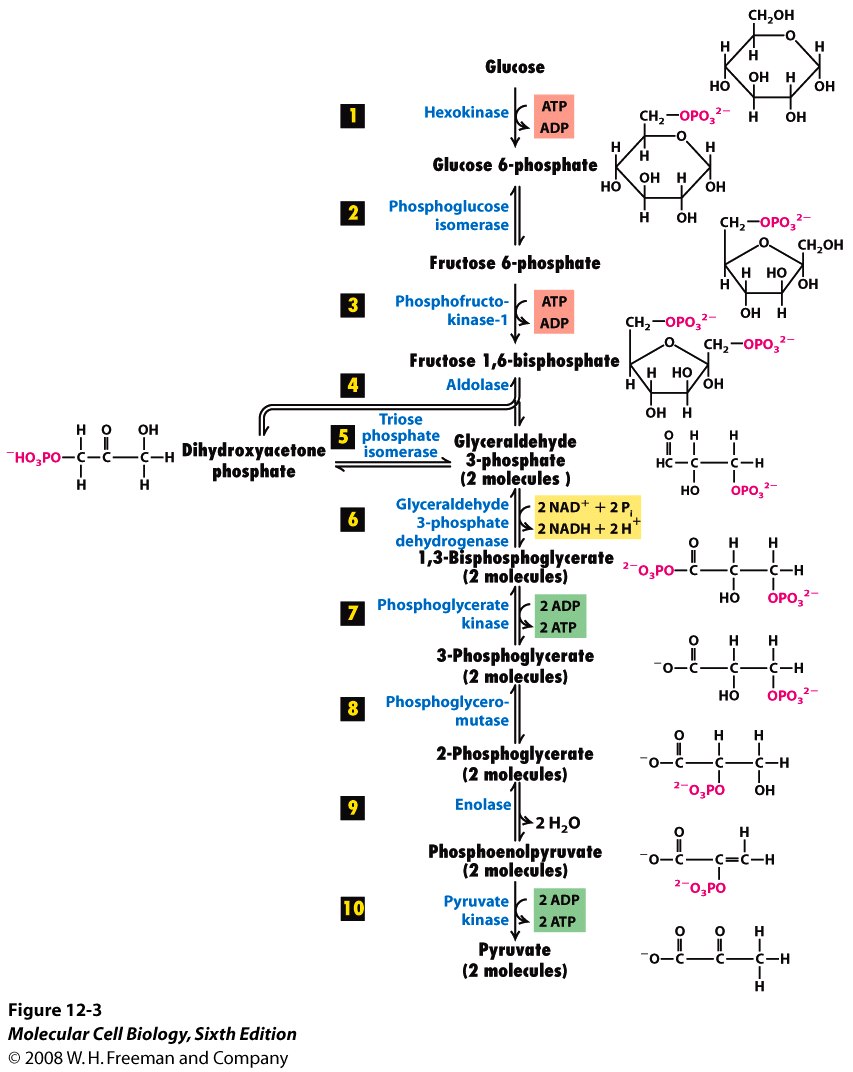
If your eyes tend to glaze over when looking at this, don’t feel bad—so do mine. There’s a lot of information here. But if you look carefully, you’ll see that the 1st and 3rd stages of glycolysis actually convert 2 ATP’s to ADP, while the 7th and 10th convert 4 ADP’s to ATP. So, the early steps require free energy, while the later ones double this investment. As the saying goes, “it takes money to make money”.
This nuance makes it clear that if a cell starts with no ATP, it won’t be able to make ATP by glycolysis. And if has just a small amount of ATP, it won’t be very good at making it this way.
In short, this affects the dynamics in an important way. But I don’t see how it could explain oscillations in how much ATP is manufactured from a constant supply of glucose!
We can look up the free energy changes for each of the 10 reactions in glycolysis. Here they are, named by the enzymes involved:

I got this from here:
• Leslie Frost, Glycolysis.
I think these are her notes on Chapter 14 of Voet, Voet, and Pratt’s Fundamentals of Biochemistry. But again, I don’t think these explain the oscillations. So we have to look elsewhere.
Oscillations
By some careful detective work—by replacing the input of glucose by an input of each of the intermediate products—biochemists figured out which step causes the oscillations. It’s the 3rd step, where fructose-6-phosphate is converted into fructose-1,6-bisphosphate, powered by the conversion of ATP into ADP. The enzyme responsible for this step is called phosphofructokinase or PFK. And it turns out that PFK works better when there is ADP around!
In short, the reaction network shown above is incomplete: ADP catalyzes its own formation in the 3rd step.
How does this lead to oscillations? The Higgins–Selkov model is a scenario for how it might happen. I’ll explain this model, offering no evidence that it’s correct. And then I’ll take you to a website where you can see this model in action!
Suppose that fructose-6-phosphate is being produced at a constant rate. And suppose there’s some other reaction, which we haven’t mentioned yet, that uses up ADP at a constant rate. Suppose also that it takes two ADP’s to catalyze the 3rd step. So, we have these reactions:
fructose-6-phosphate + 2 ADP → 3 ADP
ADP →
Here the blanks mean ‘nothing’, or more precisely ‘we don’t care’. The fructose-6-biphosphate is coming in from somewhere, but we don’t care where it’s coming from. The ADP is going away, but we don’t care where. We’re also ignoring the ATP that’s required for the second reaction, and the fructose-1,6-bisphosphate that’s produced by this reaction. All these features are irrelevant to the Higgins–Selkov model.
Now suppose there’s initially a lot of ADP around. Then the fructose-6-phosphate will quickly be used up, creating even more ADP. So we get even more ADP!
But as this goes on, the amount of fructose-6-phosphate sitting around will drop. So, eventually the production of ADP will drop. Thus, since we’re positing a reaction that uses up ADP at a constant rate, the amount of ADP will start to drop.
Eventually there will be very little ADP. Then it will be very hard for fructose-6-phosphate to get used up. So, the amount of fructose-6-phosphate will start to build up!
Of course, whatever ADP is still left will help use up this fructose-6-phosphate and turn it into ADP. This will increase the amount of ADP. So eventually we will have a lot of ADP again.
We’re back where we started. And so, we’ve got a cycle!
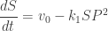
Of course, this story doesn’t prove anything. We should really take our chemical reaction network and translate it into some differential equations for the amount of fructose-6-phosphate and the amount of ADP. In the Higgins–Selkov model people sometimes write just ‘S’ for fructose-6-phosphate and ‘P’ for ADP. (In case you’re wondering, S stands for ‘substrate’ and P stands for ‘product’.) So, our chemical reaction network becomes
S + 2P → 3P
P →
and using the law of mass action we get these equations:

where 


Now we can solve these differential equations and see if we get oscillations. The answer depends on the constants
To see what actually happens, try this website:
• Mike Martin, Glycolytic oscillations: the Higgins–Selkov model.
If you run it with the constants and initial conditions given to you, you’ll get oscillations. You’ll also get this vector field on the 

This is called a phase portrait, and its a standard tool for studying first-order differential equations where two variables depend on time.
This particular phase portrait shows an unstable fixed point and a limit cycle. That’s jargon for saying that in these conditions, the system will tend to oscillate. But if you adjust the constants, the limit cycle will go away! The appearance or disappearance of a limit cycle like this is called a Hopf bifurcation.
For details, see:
• Alan Rendall, Dynamical systems, Chapter 11: Oscillations.
He shows that the Higgins–Selkov model has a unique stationary solution (i.e. fixed point), which he describes. By linearizing it, he finds that this fixed point is stable when 
In the unstable case, if the solutions are all bounded as 
• Alan Rendall, The Higgins–Selkov oscillator.


Thanks a lot for the nice picture of storm petrels. It is interesting that apparently the experimental work on glycolytic oscillations was stimulated by mathematical modelling. Here is a quote from the web page of Evgeni Selkov
(http://www.mcs.anl.gov/~pieper/selkovsr.html):
Thanks! It’s really fascinating that theory, and ideas about electrical circuits, led experiment in this case. May it do so again!
Here’s one big question I failed to ask in my post: is there some ‘good reason’ why the third reaction uses ADP to help catalyze the production of ADP? One might wonder if a feedback mechanism of this sort plays a useful role in the cell. Perhaps the oscillations are useful, or perhaps they’re just a consequence of something else that’s useful.
Or, perhaps this feedback loop is just a ‘coincidence’.
In his book Goldbeter makes some remarks on the usefulness of glycolytic oscillations and apparently they are not known to be useful to the yeast. But they might be useful to us. Insulin is secreted in an oscillatory manner and there is an idea due to Keith Tornheim that these may be driven by glycolytic oscillations in the cells producing insulin. The oscillations in insulin levels are disrupted in some patients with Type 2 diabetes and this may be due to a mutation in the gene for PFK.
“If your eyes tend to glaze over when looking at this…”. Now you know how I feel.
The figure (12.3 from MCB, 6th Edition.) is rich in information if you know the code: kinase, isomerase, mutase, aldolase, enolase are not random names – they describe specific functions. The reactions are invariably stereospecific. Some reactions may proceed in vitro, but enzyme catalysis imparts stereospecificity. Enzymes are often part of multi-protein complexes and may require co-factors (Mg2+ in this example)
In the case of NAD, the “little plus sign” is located on a quaternary nitrogen – four bonds instead of the usual three for nitrogen (cf the -NH2). So, the two O-s have no bearing on the matter, other than making the overall charge -1. You can’t write a quaternary nitrogen as ‘neutral’. On reduction, the hydrogen can in principle come in from either side of the nicotinamide ring, and reduction to NADH may be stereospecific (I haven’t checked). Ideally one would draw the NAD/NADH molecule without the ‘extended’ anhydride bridge (-P-O-P-). Using Rasmol or some other free 3D-modelling tool would provide a better idea of the 3D-shape. It’s worth mentioning that NADH is fluorescent and allows reactions to be followed.
I found this set of teaching slides on “Glycolytic Oscillations” of interest – the insulin oscillation is mentioned as well as the Sel’kov and later models (with references). You also get some experimental chart data!!
Apologies if the comment appears in the wrong place, it can be confusing …
Professor Baez wrote: “Glycolysis actually consists of 10 steps, each mediated by its own enzyme.” My question, have all ten enzymes been rigorously proven, say by sequential analysis of their amino acids? A ten step metabolic pathway might also be explained as a ten column binomial distribution due to the energy of the system being available to the participating molecules as quanta. Black Body radiation presents to the experimental physicist as a bell shaped distribution with skew. This is obviously a binomial with so many energy levels the columns take on the appearance of a smooth bell shaped curve. (The Limit Concept) Might the many step processes so common in biochemistry have the same explanation as Black Body Radiation?
You can see the ten enzymes at https://en.wikipedia.org/wiki/Glycolysis. They’re in pink from about a quarter way down. I bet they’ve been sequenced 100s of times in different organisms, and their 3D structure found.
One reason for having many steps in biochemistry is that collecting energy from one big step is difficult, like running a waterwheel from Niagra Falls. The enzymes turn this into ten little waterfalls.
Dear Graham- Thanks for the link. My skepticism stems from the fact biologists and biochemists are math illiterates, prone to miss interpreting their phenomena. They invariably break down a logistic equilibrium (The Sigmoid S Shaped Curve) into three artificial phases: (1) lag (2) linear and (3) exponential or logarithmic. Next they invoke mysterious control substances to explain away the change in curvature with elapsed time. As you know, a process characterized by a symmetrical sigmoid curve is merely reversible, nothing more, nothing less. Thanks again. And if I may be so bold, ten little waterfalls might be better described as a binomial composed of ten columns.
I think I am settling into this open source research environment.
Chemistry and biochemistry use advanced math. (Admittedly they may lure physicists to help, but they are the exceptions that prove the rule.)
The previous article has (at least) a long recent comment that goes into control of first and last steps of a typical ~ 10 step metabolic pathway like glycolysis, and other reasons for steps such as substrate handling. (Remember, metabolism is both energy and matter (molecule, electron) transformations, i.e. an energy only description won’t capture it.)
There are more reasons to divide and conquer. The matching of energies becomes easier, in fact chemiosmosis divides even finer to pump ‘protons’ (actually H3O+) over the inner cell membrane to scrounge out energy differentials. Likely a less efficient cell would not be a problem, after all the UCA lineage did not evolve chemiosmosis early. (Need a complicated ATP producing molecular machine based on proteins, instead of glycolysis cytoplasm ATP generation.) But notably chemiosmosis was present in the LUCA and all other cell types have gone extinct or possibly evolved into metabolic free viruses. “That’s not a knife. THAT’s a knife.”
Great! It’s good having you here.
(I hope to give a more intelligent reply later.)
This articles has a link to a website that simulates glycolytic oscillations:
• Mike Martin, Glycolytic oscillations: the Higgins–Selkov model.
I’d like to see more such things, since I’m looking at a lot of chemical reaction networks these days. I don’t need these programs for my own research—not yet, anyway. But they would be very nice to explain my research.
After I wrote this article, in just a couple hours Dara Shayda created a demo that relies on the Wolfram Cloud:
• Dara Shayda, Glycolytic oscillations: the Higgins–Selkov model.
I believe Mike Martin’s webpaage relies on Mathematica too.
It’s great that Dara can create such a page so fast. I could add text to this and turn it into a nice little introduction to this model of glycolytic oscillations. How could we make it even nicer?
Both these websites require that you type in some numbers. It would be more intuitive to use sliders. Dara had created a website that uses sliders, but the latency makes it very frustrating to use: you can try to slide the slider, but it just sits there for a while!
Using Javascript, some of the Azimuth gang made a webpage that works on my website, uses sliders to take inputs, and uses your browser to run a simple climate model in real time:
• Michael Knap and Taylor Baldwin, A simple stochastic energy balance model.
It looks and feels great. I get the feeling that main reason people don’t do more of these is that people hate doing math programming in Javascript.
So, there seems to be some tradeoff between what’s quick and easy to program (which is very important) and what feels nice to the user.
Here I am only interested in things that end users can run, using a web browser or maybe even a mobile phone, without downloading any special software.
On the Azimuth Forum, WebHubTel replied:
Yes, Dara mentioned that downloading the CDF Player would allow me to use sliders without the annoying time lag. But I never download software unless I’m quite committed to a project. I wouldn’t do it if I just bumped into someone’s website while trying to learn about something. I figure there are lots of people like me. So, I’d like to see educational software that works for people like me.
If I needed to simulate chemical reaction networks for my own research, of course I would download software to do it. But I haven’t needed this yet.
Over on the Azimuth Forum, Daniel Mahler wrote:
I have made some improvements to the notebook at http://mybinder.org/repo/mhlr/notebooks/Higgins-Selkov.ipynb
“Puzzle 1. Why does NAD+ have a little plus sign on it, despite the two O–’s in the picture above?”
I think it was in one of the MOOC biochemistry courses I took in order to get a similar overview. It is a formalism that connote the difference between physiological pH and one of the extreme ways of estimating a pH effect (electron placement). I don’t have the energy to look up the course, but Wikipedia was helpful for a lazyman:
“Although NAD+ is written with a superscript plus sign because of the formal charge on a particular nitrogen atom, at physiological pH for the most part it is actually a singly charged anion (charge of minus 1), while NADH is a doubly charged anion.” [ https://en.wikipedia.org/wiki/Nicotinamide_adenine_dinucleotide ; https://en.wikipedia.org/wiki/Formal_charge ]
By the way, the same problem with placing electrons as an effect of pH (mostly) is shared with how the enzymes behaves.
“Puzzle 2. There is often roughly 700 times as much NAD+ as NADH in the cytoplasm of mammals. In these conditions, what is the free energy difference between NAD+ and NADH? I think this is something you’re supposed to be able to figure out.”
Right, if we can assume that there is an equlibrium the reaction constants should be an expression of chemical potentials, i.e. a derivative of the free energy. Specifically the c.p.’s should sum to 0 (equilibrium), so the free energy is minimized. I don’t know if it is helpful. (But I note that if one approximates the system with a binary mixture at equilibrium, the ratio of free energies relates as the ratio between species.)
(Oops, it is the ratio of derivatives of c.p.’s that relates that way, so it is a double derivative of free energies. Need more constraints then. :-/)
Torbjörn cited Wikipedia’s answer to Puzzle 1:
Nice! That was helpful. I had a less profound answer to Puzzle 1.
If you look carefully at this picture of NAD+, you’ll see a little plus sign. That little plus sign is not there in NADH. That’s the difference between NAD+ and NADH.
Regarding this:
I believe the difference in Gibbs free energies is related to the ratio of concentrations
  in equilibrium as follows:
Here is measured in joules per mole,
  is a dimensionless quantity, where both
  and
and  are measured in moles per liter,
  is the temperature in kelvin and
  is the gas constant, 8.31446 joules per kelvin per mole.
If this is right, and if we can treat NAD+ and NADH as approximately in equilibrium, we can figure out their difference in free energies.
You lost me here: “1st and 3rd stages of glycolysis actually convert 2 ATP’s to ADP, while the 7th and 10th convert 4 ADP’s to ATP.” I see the same number of ADPs and ATPs on both sides in those steps.
See below how reactions 5-10 all say “2 molecules” under them? That’s because reaction 5 splits a 6-carbon molecule into two 3-carbon molecules. So, everything after this point is doubled!
Hmm, but maybe that’s not what you were complaining about. Maybe you’re telling me I should have said this:
“The 1st and 3rd stages of glycolysis actually convert a total of 2 ATP’s to 2 ADP’s, while the 7th and 10th convert a total of 4 ADP’s to 4 ATP’s.”
That’s what I meant. Is that the problem?
It’s actually reaction 4 that does the split. Reaction 5 converts dihydroxyacetone phosphate into glyceraldehye-3-phosphate, which is the starting point for the subsequent steps, starting with step 6.
Whoops, I could have seen that. I got confused by the “detour” in the chart above. I guess that detour means this part of the reaction can proceed in two steps or one.
Not sure if I’ve understood you correctly, but reaction 4 has two products, drawn side by side. The numeral “4” is just hovering in the general vicinity of the relevant arrows. Reaction 5 converts one of those products to be the same as the other.
Oh. So the branching arrows are not alternative choices for how reaction 4 can proceed: fructose 1,6-biphosphate turns into dihydroxyacetone phosphate and glyceraldehyde 3-phosophate, not or.
I could easily have seen this must be so, using conservation of carbon, but I tend to not really look at the details of reactions like this, thinking “this is too complicated for me”.
A small correction: the second equation should say , not
, not  .
.
I thought that having to reload the page for a new set of values was too tiring, so I sketched a somewhat simpler, but a bit more interactive simulator.
Thanks for catching that mistake! It’s fixed now.
I don’t see the simulation, just the differential equations and partial equations like
I don’t seem able to enter values for these variables. Enabling cookies didn’t help.
I am very eager to see more interactive simulators that people can run simply by visiting a website.
Hmm, interesting, it’s means that somehow some of the JavaScript doesn’t load for you. Can you check JavaScript console for any error messages? What’s the browser you are using? (I developed on Chrome 48.0.2564.81, but there’s nothing the older version shouldn’t be able to deal with.)
I made a small change to the JS that should probably improve compatibility with older browsers, hopefully that helps.
As a side note, the ODE solver library that I’m using is not very flexible, so unfortunately I can’t control the step size directly. It also for some reason fails to produce any solution for some combinations of input and T (increasing T to 90 caused it to fail for me, so I limited to 80, but some combinations of values can probably still break it).
I thought of making a real phase portrait picture, but doing it right and making it pretty is a bit tricky, so that’s something for another time.
I’m using Firefox 43.0.4 on a Windows laptop. Luckily, whatever you did fixed the problem—your simulator is working for me now.
What is T? The reciprocal of the time step?
I’m integrating from 0 to T. It doesn’t seem to affect the time step much (except for the case of a very small T), as far as I understand the step is limited by the max error value that I pass as an argument to the solver.
I’m a bit rusty on the stability theory: isn’t the fixed point stable in the Lyapunov sense (you say it’s unstable in the text)? For any there exists a region, where for any starting point
  from that region the solution would tend to the fixed point, and would stay closer than
  to the fixed point. You probably even have absolute stability.
I haven’t studied the stability myself, so I could be wrong, but Alan studied it in these course notes:
• Alan Rendall, Dynamical systems, Chapter 11: Oscillations.
He shows that the Higgins–Selkov model has a unique stationary solution (i.e. fixed point), which he describes. By linearizing it, he finds that this fixed point is stable when (the inflow of the ‘substrate’ S) is less than a certain value, and unstable when it exceeds that value.
In the unstable case, if the solutions are all bounded as there must be a periodic solution. In the course notes he shows this is indeed what happens in a simpler model of glycolysis, the Schnakenberg model. In some separate notes he shows it for the Higgins–Selkov model, at least for certain values of the parameters:
• Alan Rendall, The Higgins–Selkov oscillator.
The proof here seems complicated, and I would hope it could be simplified using some additional ideas… but I haven’t tried, and Alan is the expert on this, not me.
OK, so if I understand it correctly, the particular phase portrait that you used above is actually for a stable stationary solution case: the solutions in the vicinity of the fixed point (look like they) are not periodic, and thus tend to the fixed point for . You however say that it is unstable, which, as I am a bit more convinced now, is wrong, if we take the visual behavior of this plot at face value. As far as I understand, this is the plot for
  , which is indeed unstable according to the formula, however the error accumulation during numerical integration with these parameters causes the solution to veer off slightly closer to the fixed point, thus making this into a phase portrait of a stable case. I’m afraid it’d be a bit tricky to produce a plot for the (rather interesting!) unstable case with the periodic solutions using naive numeric integration.
I added plotting of the fixed point to my visualization, however, quite surprisingly, it seems that it doesn’t match what the plotted ODE solution behavior for some of sets of parameters (try ). Choosing the fixed point as a starting point shows a non-stationary solution, and, after having double-checked my code I suspect that the ODE solver that I’m using is not very good (though there is still some chance that I screwed up something).
Ah, I indeed had a typo in fixed point computation, that is fixed, and everything looks a bit more reasonable now.
Great! Analytical results are a good way to check ones programming.
The fixed point of the Higgins–Selkov model is stable if
and unstable if
The picture in my blog shows Martin’s calculation for
 So, in fact this case should be stable, though very close to becoming unstable. So, my blog article was wrong in stating that it’s unstable!
I need to think about this a bit more….
Hi John,
There’s a small mistake in your analysis of the stability of the fixed point of the Higgins-Selkov system. In one of your comments above, you stated that the fixed point is stable if
and unstable if
The correct condition should be that it’s stable if
and unstable if
(Note the reversed inequalities, and the different exponents on the right hand side.) So what you stated in the article about the system having a limit cycle attractor for larger values of is backwards as well.
It’s for this reason that the system shown in Mike Martin’s default example (with ) has a limit cycle attractor, i.e. the fixed point is in fact unstable there. While it is “barely” unstable there, the simulations I’ve been doing show that this system needs to be “barely” unstable like that in order to have a limit cycle attractor. I initially varied the parameters by somewhat large increments, and the behavior quickly became unbounded. This is explained pretty well in Rendall’s notes on it (the last link in your article).
By the way, thanks for this article. I’m using it as an example (in fact, a homework exercise) in my nonlinear dynamics class for biologists.
Thanks for the correction! I’m inclined to believe you even before checking, because the computer simulations seemed to be acting funny. I hadn’t checked the formulas myself; I just copied them down from somewhere, and it seems I either copied them wrong or my source had a mistake.
I’ll try to fix this, but I’m tempted to check first!
I think that it’s also worth noting that while the original Higgins-Selkov model has three control parameters (which I think have nice biological meaning), after the non-dimensionalization procedure the system has only one parameter. It’s easier to study system with only one parameter and it becomes more apparent what bifurcations might happen. (Frankly speaking, only Andronov-Hopf bifurcation happens…)
Good point! Since the Higgins–Selkov model involves just 2 functions of time, we can use the Poincaré–Bendixson theorem to limit the options for its qualitative behavior at any value of the parameter you mention:
There must be some theorem explaining what catastrophes can happen in this situation if we smoothly vary the system in a way that depends on a single parameter… at least in the generic cases. But I don’t know that theorem.
Clearly Hopf bifurcations are the most famous of these catastrophes.
Well, there is a list of codimension one bifurcations (they are partially listed here http://www.scholarpedia.org/article/Bifurcation#Classification_of_bifurcations, for example).
Having only one parameter restricts equilibria bifurcations to three generic possibilities: Andronov-Hopf, saddle-node (roughly, two equilibria collide and disappear) and pitchfork bifurcations (like, stable equilibrium becomes unstable and spawns two stable equilibria; it happens when system has symmetry and thus it’s less generic). In nice (and, possibly, simple) cases bifurcation set is a finite union of hypersurfaces in parameter space; other bifurcation points belong to subsets of codimension greater than 1, but they still belong to this union of hypersurfaces. So this illustrates why it is more likely that we hit Andronov-Hopf/saddle-node/pitchfork bifurcation than any other.
The codimension one bifurcations were the ones I wanted, since these are precisely the ones a generic path in the parameter space will hit. Thanks!
Posting a link to an R-based example of modeling glycolysis. My non-mathematician quick read is that it doesn’t involves solving nonlinear systems since I think the differential equations being used are linear, but the methods might be useful for modeling resource constraints.
“Escherichia coli Core Metabolism Model in LIM” by Karline Soetaert
Click to access LIMecoli.pdf
After a long time I finally did a more extensive analysis of Selkov’s model of glycolysis together with my student Pia Brechmann. We wrote a paper on this
https://arxiv.org/abs/1803.10579
and there is a short introduction on my blog
Great, thanks! By chance, next week I’m going to visit Gheorghe Craciun at the University of Wisconsin, to talk about chemical reaction networks. But I haven’t thought about Selkov’s model for a long time, so I’ll need to revive my dormant memories. I’m glad you figured out more about it!