Large Countable Ordinals (Part 1)

I love the infinite.

It may not exist in the physical world, but we can set up rules to think about it in consistent ways, and then it’s a helpful concept. The reason is that infinity is often easier to think about than very large finite numbers.

Finding rules to work with the infinite is one of the great triumphs of mathematics. Cantor’s realization that there are different sizes of infinity is truly wondrous—and by now, it’s part of the everyday bread and butter of mathematics.

Trying to create a notation for these different infinities is very challenging. It’s not a fair challenge, because there are more infinities than expressions we can write down in any given alphabet! But if we seek a notation for countable ordinals, the challenge becomes more fair.

It’s still incredibly frustrating. No matter what notation we use it fizzles out too soon… making us wish we’d invented a more general notation. But this process of ‘fizzling out’ is fascinating to me. There’s something profound about it. So, I would like to tell you about this.

Today I’ll start with a warmup. Cantor invented a notation for ordinals that works great for ordinals less than a certain ordinal called ε₀. Next time I’ll go further, and bring in the ‘single-variable Veblen hierarchy’! This lets us describe all ordinals below a big guy called the ‘Feferman–Schütte ordinal’.

In the post after that I’ll bring in the ‘multi-variable Veblen hierarchy’, which gets us all the ordinals below the ‘small Veblen ordinal’. We’ll even touch on the ‘large Veblen ordinal’, which requires a version of the Veblen hierarchy with infinitely many variables. But all this is really just the beginning of a longer story. That’s how infinity works: the story never ends!

To describe countable ordinals beyond the large Veblen ordinal, most people switch to an entirely different set of ideas, called ‘ordinal collapsing functions’. I may tell you about those someday. Not soon, but someday. My interest in the infinite doesn’t seem to be waning. It’s a decadent hobby, but hey: some middle-aged men buy fancy red sports cars and drive them really fast. Studying notions of infinity is cooler, and it’s environmentally friendly.

I can even imagine writing a book about the infinite. Maybe these posts will become part of that book. But one step at a time…

Cardinals versus ordinals

Cantor invented two different kinds of infinities: cardinals and ordinals. Cardinals say how big sets are. Two sets can be put into 1-1 correspondence iff they have the same number of elements—where this kind of ‘number’ is a cardinal. You may have heard about cardinals like aleph-nought (the number of integers), 2 to power aleph-nought (the number of real numbers), and so on. You may have even heard rumors of much bigger cardinals, like ‘inaccessible cardinals’ or ‘super-huge cardinals’. All this is tremendously fun, and I recommend starting here:

• Frank R. Drake, Set Theory, an Introduction to Large Cardinals, North-Holland, 1974.

There are other books that go much further, but as a beginner, I found this to be the most fun.

But I don’t want to talk about cardinals! I want to talk about ordinals.

Ordinals say how big ‘well-ordered’ sets are. A set is well-ordered if it comes with a relation ≤ obeying the usual rules:

• Transitivity: if x ≤ y and y ≤ z then x ≤ z

• Reflexivity: x ≤ x

• Antisymmetry: if x ≤ y and y ≤ x then x = y

and one more rule: every nonempty subset has a smallest element!

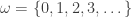
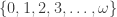
For example, the empty set

$\{\}$

is well-ordered in a trivial sort of way, and the corresponding ordinal is called

$0$

Similarly, any set with just one element, like this:

$\{0\}$

is well-ordered in a trivial sort of way, and the corresponding ordinal is called

$1$

Similarly, any set with two elements, like this:

$\{0,1\}$

becomes well-ordered as soon as we decree which element is bigger; the obvious choice is to say 0 < 1. The corresponding ordinal is called

$2$

Similarly, any set with three elements, like this:

$\{0,1,2\}$

becomes well-ordered as soon as we linearly order it; the obvious choice here is to say 0 < 1 < 2. The corresponding ordinal is called

$3$

Perhaps you're getting the pattern — you've probably seen these particular ordinals before, maybe sometime in grade school. They're called finite ordinals, or "natural numbers".

But there's a cute trick they probably didn't teach you then: we can define each ordinal to be the set of all ordinals less than it:

$0 = \{\}$ (since no ordinal is less than 0)
$1 = \{0\}$ (since only 0 is less than 1)
$2 = \{0,1\}$ (since 0 and 1 are less than 2)
$3 = \{0,1,2\}$ (since 0, 1 and 2 are less than 3)

and so on. It’s nice because now each ordinal is a well-ordered set of the size that ordinal stands for. And, we can define one ordinal to be “less than or equal” to another precisely when its a subset of the other.

Infinite ordinals

What comes after all the finite ordinals? Well, the set of all finite ordinals is itself well-ordered:

$\{0,1,2,3,\dots \}$

So, there’s an ordinal corresponding to this — and it’s the first infinite ordinal. It’s usually called $\omega,$ pronounced ‘omega’. Using the cute trick I mentioned, we can actually define

$\omega = \{0,1,2,3,\dots\}$

What comes after this? Well, it turns out there’s a well-ordered set

$\{0,1,2,3,\dots,\omega\}$

containing the finite ordinals together with $\omega,$ with the obvious notion of “less than”: $\omega$ is bigger than the rest. Corresponding to this set there’s an ordinal called

$\omega+1$

As usual, we can simply define

$\omega+1 = \{0,1,2,3,\dots,\omega\}$

At this point you could be confused if you know about cardinals, so let me throw in a word of reassurance. The sets $\omega$ and $\omega+1$ have the same cardinality: they are both countable. In other words, you can find a 1-1 and onto function between these sets. But $\omega$ and $\omega+1$ are different as ordinals, since you can’t find a 1-1 and onto function between them that preserves the ordering. This is easy to see, since $\omega+1$ has a biggest element while $\omega$ does not.

Indeed, all the ordinals in this series of posts will be countable! So for the infinite ones, you can imagine that all I’m doing is taking your favorite countable set and well-ordering it in ever more sneaky ways.

Okay, so we got to $\omega + 1.$ What comes next? Well, not surprisingly, it’s

$\omega+2 = \{0,1,2,3,\dots,\omega,\omega+1\}$

Then comes

$\omega+3, \omega+4, \omega+5,\dots$

and so on. You get the idea.

I haven’t really defined ordinal addition in general. I’m trying to keep things fun, not like a textbook. But you can read about it here:

• Wikipedia, Ordinal arithmetic: addition.

The main surprise is that ordinal addition is not commutative. We’ve seen that $\omega + 1 \ne \omega,$ since

$\omega + 1 = \{0, 1, 2, 3, \dots, \omega \}$

is an infinite list of things… and then one more thing that comes after all those!. But $1 + \omega = \omega,$ because one thing followed by a list of infinitely many more is just a list of infinitely many things.

With ordinals, it’s not just about quantity: the order matters!

ω+ω and beyond

Okay, so we’ve seen these ordinals:

$1, 2, 3, \dots, \omega, \omega + 1, \omega + 2, \omega+3, \dots$

What next?

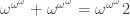
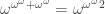
Well, the ordinal after all these is called $\omega+\omega.$ People often call it “omega times 2” or $\omega 2$ for short. So,

$\omega 2 = \{0,1,2,3,\dots,\omega,\omega+1,\omega+2,\omega+3,\dots.\}$

It would be fun to have a book with $\omega$ pages, each page half as thick as the previous page. You can tell a nice long story with an $\omega$ -sized book. I think you can imagine this. And if you put one such book next to another, that’s a nice picture of $\omega 2.$

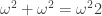
It’s worth noting that $\omega 2$ is not the same as $2 \omega.$ We have

$\omega 2 = \omega + \omega$

while

$2 \omega = 2 + 2 + 2 + \cdots$

where we add $\omega$ of these terms. But

$2 + 2 + 2 + \cdots = (1 + 1) + (1 + 1) + (1 + 1) \dots = \omega$

$2 \omega = \omega$

This is not a proof, because I haven’t given you the official definition of how to multiply ordinals. You can find it here:

• Wikipedia, Ordinal arithmetic: multiplication.

Using this you can prove that what I’m saying is true. Nonetheless, I hope you see why what I’m saying might make sense. Like ordinal addition, ordinal multiplication is not commutative! If you don’t like this, you should study cardinals instead.

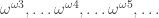
What next? Well, then comes

$\omega 2 + 1, \omega 2 + 2,\dots$

and so on. But you probably have the hang of this already, so we can skip right ahead to $\omega 3.$

In fact, you’re probably ready to skip right ahead to $\omega 4,$ and $\omega 5,$ and so on.

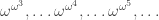
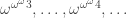
In fact, I bet now you’re ready to skip all the way to “omega times omega”, or $\omega^2$ for short:

$\omega^2 = \{0,1,2\dots\omega,\omega+1,\omega+2,\dots ,\omega 2,\omega 2+1,\omega 2+2,\dots\}$

Suppose you had an encyclopedia with $\omega$ volumes, each one being a book with $\omega$ pages. If each book is twice as thin as one before, you’ll have $\omega^2$ pages — and it can still fit in one bookshelf! Here’s the idea:

What comes next? Well, we have

$\omega^2+1, \omega^2+2, \dots$

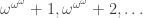
and so on, and after all these come

$\omega^2+\omega, \omega^2+\omega+1, \omega^2+\omega+2, \dots$

and so on — and eventually

$\omega^2 + \omega^2 = \omega^2 2$

and then a bunch more, and then

$\omega^2 3$

and then a bunch more, and then

$\omega^2 4$

and then a bunch more, and more, and eventually

$\omega^2 \omega = \omega^3$

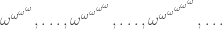
You can probably imagine a bookcase containing $\omega$ encyclopedias, each with $\omega$ volumes, each with $\omega$ pages, for a total of $\omega^3$ pages. That’s $\omega^3.$

ω^ω

I’ve been skipping more and more steps to keep you from getting bored. I know you have plenty to do and can’t spend an infinite amount of time reading this, even if the subject is infinity.

So if you don’t mind me just mentioning some of the high points, there are guys like $\omega^4$ and $\omega^5$ and so on, and after all these comes

$\omega^\omega$

Let’s try to we imagine this! First, imagine a book with $\omega$ pages. Then imagine an encyclopedia of books like this, with $\omega$ volumes. Then imagine a bookcase containing $\omega$ encyclopedias like this. Then imagine a room containing $\omega$ bookcases like this. Then imagine a floor with library with $\omega$ rooms like this. Then imagine a library with $\omega$ floors like this. Then imagine a city with $\omega$ libraries like this. And so on, ad infinitum.

You have to be a bit careful here, or you’ll be imagining an uncountable number of pages. To name a particular page in this universe, you have to say something like this:

the 23rd page of the 107th book of the 20th encyclopedia in the 7th bookcase in 0th room on the 1000th floor of the 973rd library in the 6th city on the 0th continent on the 0th planet in the 0th solar system in the…

But it’s crucial that after some finite point you keep saying “the 0th”. Without that restriction, there would be uncountably many pages! This is just one of the rules for how ordinal exponentiation works. For the details, read:

• Wikipedia, Ordinal arithmetic: exponentiation.

As they say,

But for infinite exponents, the definition may not be obvious.

Here’s a picture of $\omega^\omega,$ taken from David Madore’s wonderful interactive webpage:

On his page, if you click on any of the labels for an initial portion of an ordinal, like $\omega, \omega^2, \omega^3$ or $\omega^4$ here, the picture will expand to show that portion!

And here’s another picture, where each turn of the clock’s hand takes you to a higher power of $\omega$ :

Ordinals up to ε₀

Okay, so we’ve reached $\omega^\omega.$ Now what?

Well, then comes $\omega^\omega + 1,$ and so on, but I’m sure that’s boring by now. And then come ordinals like

$\omega^\omega 2,\dots, \omega^\omega 3, \dots, \omega^\omega 4, \dots$

leading up to

$\omega^\omega \omega = \omega^{\omega + 1}$

Then eventually come ordinals like

$\omega^\omega \omega^2 , \dots, \omega^\omega \omega^3, \dots, \omega^\omega \omega^4, \dots$

and so on, leading up to

$\omega^\omega \omega^\omega = \omega^{\omega + \omega} = \omega^{\omega 2}$

This actually reminds me of something that happened driving across South Dakota one summer with a friend of mine. We were in college, so we had the summer off, so we drive across the country. We drove across South Dakota all the way from the eastern border to the west on Interstate 90.

This state is huge — about 600 kilometers across, and most of it is really flat, so the drive was really boring. We kept seeing signs for a bunch of tourist attractions on the western edge of the state, like the Badlands and Mt. Rushmore — a mountain that they carved to look like faces of presidents, just to give people some reason to keep driving.

Anyway, I’ll tell you the rest of the story later — I see some more ordinals coming up:

$\omega^{\omega 3},\dots \omega^{\omega 4},\dots \omega^{\omega 5},\dots$

We’re really whizzing along now just to keep from getting bored — just like my friend and I did in South Dakota. You might fondly imagine that we had fun trading stories and jokes, like they do in road movies. But we were driving all the way from Princeton to my friend Chip’s cabin in California. By the time we got to South Dakota, we were all out of stories and jokes.

Hey, look! It’s

$\omega^{\omega \omega}= \omega^{\omega^2}$

That was cool. Then comes

$\omega^{\omega^3}, \dots \omega^{\omega^4}, \dots \omega^{\omega^5}, \dots$

and so on.

Anyway, back to my story. For the first half of our half of our trip across the state, we kept seeing signs for something called the South Dakota Tractor Museum.

Oh, wait, here’s an interesting ordinal:

$\omega^{\omega^\omega}$

Let’s stop and take look:

That was cool. Okay, let’s keep driving. Here comes

$\omega^{\omega^\omega} + 1, \omega^{\omega^\omega} + 2, \dots$

and then

$\omega^{\omega^\omega} + \omega, \dots, \omega^{\omega^\omega} + \omega 2, \dots, \omega^{\omega^\omega} + \omega 3, \dots$

and then

$\omega^{\omega^\omega} + \omega^2, \dots, \omega^{\omega^\omega} + \omega^3, \dots$

and eventually

$\omega^{\omega^\omega} + \omega^\omega$

and eventually

$\omega^{\omega^\omega} + \omega^{\omega^\omega} = \omega^{\omega^\omega} 2$

and then

$\omega^{\omega^\omega} 3, \dots, \omega^{\omega^\omega} 4, \dots, \omega^{\omega^\omega} 5, \dots$

and eventually

$\omega^{\omega^\omega} \omega = \omega^{\omega^\omega + 1}$

After a while we reach

$\omega^{\omega^\omega+2},\dots, \omega^{\omega^\omega+3},\dots,\omega^{\omega^\omega+4},\dots$

and then

$\omega^{\omega^\omega + \omega}, \dots, \omega^{\omega^\omega + \omega 2}, \dots, \omega^{\omega^\omega + \omega 3}, \dots$

and then

$\omega^{\omega^\omega + \omega^2}, \dots, \omega^{\omega^\omega + \omega^3}, \dots, \omega^{\omega^\omega + \omega^4}, \dots$

and then

$\omega^{\omega^\omega + \omega^\omega} = \omega^{\omega^\omega 2}$

and then

$\omega^{\omega^\omega 3}, \dots, \omega^{\omega^\omega 4} , \dots$

and then

$\omega^{\omega^\omega \omega} = \omega^{\omega^{\omega + 1}}$

and eventually

$\omega^{\omega^{\omega + 2}}, \dots, \omega^{\omega^{\omega + 3}}, \dots, \omega^{\omega^{\omega + 4}}, \dots$

This is pretty boring; we’re already going infinitely fast, but we’re still just picking up speed, and it’ll take a while before we reach something interesting.

Anyway, we started getting really curious about this South Dakota Tractor Museum — it sounded sort of funny. It took 250 kilometers of driving before we passed it. We wouldn’t normally care about a tractor museum, but there was really nothing else to think about while we were driving. The only thing to see were fields of grain, and these signs, which kept building up the suspense, saying things like

ONLY 100 MILES TO THE SOUTH DAKOTA TRACTOR MUSEUM!

We’re zipping along really fast now:

$\omega^{\omega^{\omega^\omega}}, \dots, \omega^{\omega^{\omega^{\omega^\omega}}},\dots , \omega^{\omega^{\omega^{\omega^{\omega^{\omega}}}}},\dots$

What comes after all these?

At this point we need to stop for gas. Our notation for ordinals just ran out!

The ordinals don’t stop; it’s just our notation that fizzled out. The set of all ordinals listed up to now — including all the ones we zipped past — is a well-ordered set called

$\epsilon_0$

or “epsilon-nought”. This has the amazing property that

$\epsilon_0 = \omega^{\epsilon_0}$

And it’s the smallest ordinal with this property! It looks like this:

It’s an amazing fact that every countable ordinal is isomorphic, as an well-ordered set, to some subset of the real line. David Madore took advantage of this to make his pictures.

Cantor normal form

I’ll tell you the rest of my road story later. For now let me conclude with a bit of math.

There’s a nice notation for all ordinals less than $\epsilon_0,$ called ‘Cantor normal form’. We’ve been seeing lots of examples. Here is a typical ordinal in Cantor normal form:

$\omega^{\omega^{\omega^{\omega+\omega+1}}} \; + \; \omega^{\omega^\omega+\omega^\omega} \; + \; \omega^\omega \;+\; \omega + \omega + 1 + 1 + 1$

The idea is that you write it out using just + and exponentials and 1 and $\omega.$

Here is the theorem that justifies Cantor normal form:

Theorem. Every ordinal $\alpha$ can be uniquely written as

$\alpha = \omega^{\beta_1} c_1 + \omega^{\beta_2}c_2 + \cdots + \omega^{\beta_k}c_k$

where $k$ is a natural number, $c_1, c_2, \ldots, c_k$ are positive integers, and $\beta_1 > \beta_2 > \cdots > \beta_k \geq 0$ are ordinals.

It’s like writing ordinals in base $\omega.$

Note that every ordinal can be written this way! So why did I say that Cantor normal form is nice notation for ordinals less than $\epsilon_0$ ? Here’s the problem: the Cantor normal form of $\epsilon_0$ is

$\epsilon_0 = \omega^{\epsilon_0}$

So, when we hit $\epsilon_0,$ the exponents $\beta_1 ,\beta_2, \dots, \beta_k$ can be as big as the ordinal $\alpha$ we’re trying to describe! So, while the Cantor normal form still exists for ordinals $\geq \epsilon_0,$ it doesn’t give a good notation for them unless we already have some notation for ordinals this big!

This is what I mean by a notation ‘fizzling out’. We’ll keep seeing this problem in the posts to come.

But for an ordinal $\alpha$ less than $\epsilon_0,$ something nice happens. In this case, when we write

$\alpha = \omega^{\beta_1} c_1 + \omega^{\beta_2}c_2 + \cdots + \omega^{\beta_k}c_k$

all the exponents $\beta_1, \beta_2, \dots, \beta_k$ are less than $\alpha.$ So we can go ahead and write them in Cantor normal form, and so on… and because ordinals are well-ordered, this process ends after finitely many steps.

So, Cantor normal form gives a nice way to write any ordinal less than $\epsilon_0$ using finitely many symbols! If we abbreviate $\omega^0$ as $1,$ and write multiplication by positive integers in terms of addition, we get expressions like this:

$\omega^{\omega^{\omega^{\omega^{1 + 1} +\omega+1}}} \; + \; \omega^{\omega^\omega+\omega^\omega} \; + \; \omega^{\omega+1+1} \;+\; \omega + 1$

They look like trees. Even better, you can write a computer program that does ordinal arithmetic for ordinals of this form: you can add, multiply, and exponentiate them, and tell when one is less than another.

So, there’s really no reason to be scared of $\epsilon_0.$ Remember, each ordinal is just the set of all smaller ordinals. So you can think of $\epsilon_0$ as the set of tree-shaped expressions like the one above, with a particular rule for saying when one is less than another. It’s a perfectly reasonable entity. For some real excitement, we’ll need to move on to larger ordinals. We’ll do that next time.

For more, see:

• Wikipedia, Cantor normal form.

This entry was posted on Wednesday, June 29th, 2016 at 1:00 am and is filed under mathematics. You can follow any responses to this entry through the RSS 2.0 feed. You can leave a response, or trackback from your own site.

76 Responses to Large Countable Ordinals (Part 1)

Marek14 says:

29 June, 2016 at 6:18 am

Well, the part of large ordinals I like is the theorem that states that for every increasing function f(x) with certain properties there is a fixed point — an ordinal a such that f(a) = a. Epsilon is the smallest fixed point of omega^x, but function that assigns epsilon-x to x (x-th ordinal with this property) also has a fixed point, function that assigns to x the x-th fixed point of THIS function has also a fixed point…

Reply
- John Baez says:
  
  29 June, 2016 at 6:46 am
  
  Yes, that theorem is coming in Part 3, after lots of examples in Part 2!
  
  Reply
Carsten Führmann says:

29 June, 2016 at 7:36 am

I really enjoyed this. You are a fabulous writer, John, maybe I can learn from this.

Reply
- John Baez says:
  
  29 June, 2016 at 11:02 pm
  
  Thanks! I have some tricks for writing, which I should explain someday. I started writing a paper about this:
  
  • Why mathematics is boring.
  
  but I got bored and never finished it.
  
  Reply
  - Carsten Führmann says:
    
    5 July, 2016 at 7:54 pm
    
    Thanks for the reference! It turns out that your text is a clearer, more eloquent version of principles I figured out over the years, but haven’t completely mastered for lack of practice. But here is something that just occurred to me: if one were to write a journal paper, or a conference paper, should one maybe pretend that the reader hails from outside the field and must be seduced to read the text? Just to make things more pleasant for all involved? (I’m saying this because I still remember how tiring reviewing of papers could be.)
    
    Reply
Christopher Menzel says:

29 June, 2016 at 5:09 pm

Really enjoyable exposition. One minor terminological suggestion: Since you’ve said that cardinals measure how big sets are, it introduces an unnecessary ambiguity also to say that ordinals measure how big well-ordered sets are, since (as is clear from your exposition) the two notions of bigness come apart for infinite ordinals: ω+1 is bigger than ω in the ordinal sense but not in the cardinal sense. Perhaps it would be better to say that ordinals measure how “long” well-ordered sets are? Likewise, while you introduce the idea of one ordinal being “less than or equal to” another, you subsequently more often speak of one being smaller/bigger than another instead of being less than/greater than another. Similarly for “least/greatest”: It might be preferable, e.g., to express well-foundedness as the rule that every nonempty subset has a least (rather than smallest) element, and to say that ω+1 has a greatest (rather than biggest) element while ω does not.

You’re probably planning to offer some recommendations for further study of the ordinals, but I’ll mention two that have been very useful to me over the years: Levy’s Basic Set Theory and Devlin’s The Joy of Sets.

Reply
- Todd Trimble says:
  
  29 June, 2016 at 10:30 pm
  
  The distinction between cardinals and ordinals is also reflected in ordinary language. When we say, “one”, “two”, etc., we are referring to cardinals. When we say, “first”, “second”, etc., we are referring to ordinals. Of course Cantor went much further in clarifying what this really means.
  
  Reply
  - Abel Wolman says:
    
    30 June, 2016 at 8:27 pm
    
    Yet we don’t ordinarily say first plus first equals second, though we do identify the finite ordinals with the natural numbers.
    
    Reply
    - Todd Trimble says:
      
      1 July, 2016 at 12:13 pm
      
      So? Obviously I wasn’t trying to suggest that all aspects of ordinal arithmetic are going to be reflected in ordinary language in such a simplistic way.
      
      However, we do have the idea of placing one ordered set after another (which comes first, which comes second), as when people form a queue; this corresponds to ordinal addition. Whereas in cardinal arithmetic (a la Cantor), when we add cardinals, such a conception (which comes first, which comes second) is not the relevant matter — cardinals are treated as abstract sets, and the process is one of decategorifying the category of sets (as John has emphasized many times in various places).
  - Abel Wolman says:
    
    2 July, 2016 at 12:00 am
    
    I am burdened by a nineteenth century mentality here. I am still trying to understand what the set-theoretic conception of the natural numbers is (aware that this sort of questioning has been preempted by topos-theoretic relativism and other modern developments). As children we are taught to imagine the natural numbers as ordered, equally-spaced points on the number line. This geometric intuition still informs our thought processes as when, for example, we debate whether or not the ordinals are ‘long’ rather than ‘big,’ or when we think of cardinal and ordinal bigness as analogous to measures of weight or height (restricted, that is, to finite sets). Now, naively, I image that in ZF, or whatever set-theoretic foundations, it is sets all the way down, and therefore I have tried to locate in set theory this childhood geometric intuition. Specifically, what sets instantiate the equal spacing of the natural numbers. Finite ordinals, von Neumann’s, are strange in this regard in that they are transitive, satisfy Peano’s axioms, but seem to be unequally spaced by virtue of the definition of the successor operation. I suspect this issue (if it is one) accrues to any construction of the ordinals (natural numbers) in a set theory with an axiom of extension.
    
    As you point out, if we follow von Neumann’s ‘neat trick’ and identify cardinals with ordinals (though the trick seems necessitated by a broader foundational goal, the hierarchy of sets), then cardinality is also a nonintuitive measure of (finite) bigness since we don’t seem to have a way of saying how much bigger one cardinal is than another, that is, to reckon the spacing between sets in terms of their cardinality.
    
    When you speak of ‘abstract sets,’ you are referring, I think, to Cantor’s (and Lawvere’s) ‘lauter Einsen’ and cardinals are then his ‘Kardinalen’ formed by ‘double abstraction’ (as Christopher notes). In this case, there is indeed a notion of equal spacing in that ‘lauter Einsen’ means ‘nothing but many units’ (Lawvere, “Cohesive Toposes and Cantor’s ‘lauter Einsen'”), and one of these ‘distinct but otherwise indistingishable units’ (Christopher) can be used to define the spacing. However, as Lawever points out, Cantor’s ‘Kardinalen’ are completely different from the ‘cardinals’ discussed in most set theory texts. Zermelo found Cantor’s double abstraction construction inconsistent based as it was on distinct elements having no distinguishing properties. And while Lawvere argues for the productivity of this contradiction, I think his categorical reasoning, lovely as it is, absorbs the contradiction rather than solves it at the level of sets with extensionality: the axiom of extensionality seems to preclude the existence of unit sets. (Cantor’s ‘lauter Einsen’ also satisfy a novel statistics, but that is a different matter.)
    
    Decategorification of the category of sets has the natural numbers waiting so to speak; we descend to a familiar and well-known, albeit impoverished, mathematical object. Unfortunately, as revealed above, I am still confused about the set-theoretic nature of even this impoverished (finite) world.
    
    Reply
    - Todd Trimble says:
      
      2 July, 2016 at 12:49 pm
      
      Dear Abel: interesting though this discussion could be (and I see you’ve put a lot of thought into your remarks), I’m a little worried about hijacking the comment section by discussing philosophies of foundations, which as experience shows often continue for a long time. (I thought my initial remark about ordinals in natural language to be innocuous, but one thing leads to another…) Plus, experience shows that foundational discussions can get pretty heated, which I’d much rather avoid if possible.
      
      I’ll try to reply, but I fear this won’t be adequate. I fear in fact that everything I’m about to say is already known to you, although possibly not known to everyone reading this.
      
      Since you seem to have read Lawvere, you probably well know that he is totally opposed to the idea of “sets all the way down” with concomitant iterated membership chains, which is a signal feature of set theories based on a global membership relation, where you can take two arbitrary sets $A, B$ and always ask “ $A \in B$ ?” (In the nLab, these are called “material set theories”: one has the idea that elements of sets have themselves “substance”. As opposed to “structural set theories”, where the focus is not on what sets and their elements “are” ontologically, but what they “do” operationally, as expressed e.g. in terms of universal elements.) Lawvere rejects material set theory in part because focusing on what “elements are, really” is sterile, fruitless from a mathematician’s perspective.
      
      So what does he propose to do about it? Does he have an alternative? Again, you may well be aware of his Elementary Theory of the Category of Sets, ETCS for short, which may be viewed as a prototype structural set theory. I do think this proposal resolves the alleged contradiction brought up by Zermelo: in this axiomatic set-up, elements in and of themselves are indeed featureless. Perhaps a more accurate description is that they acquire features only in terms of their interplay within a structure, and are evidently distinct within that structure.
      
      The notion of a natural numbers object (also due to Lawvere) is a good example. Instead of attempting to say what the successor function is exactly (e.g., $s(n) = n \cup \{n\}$ or something), we simply axiomatize it, giving enough properties so that we can do recursion. In fact his definition is beautifully elegant, given in terms of a universal property that says 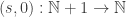$(s, 0): \mathbb{N} + 1 \to \mathbb{N}$ realizes $\mathbb{N}$ as an initial algebra of the endofunctor $X \mapsto X + 1$ (taking the coproduct with a terminal object). Being given by a universal property, $\mathbb{N}$ is uniquely determined up to uniquely specified isomorphism, which is all we ever need (or even want). I think this conception of $\mathbb{N}$ fits well with your childhood conception: the definable elements $0, s(0), ss(0), \ldots$ are equally spaced on a line, separated in unit distance by an application of $s$ . Other than their roles within the structure, these elements in and of themselves have no distinguishable features to speak of, but they are clearly distinct as part of the structure.
      
      The last question, about extensionality, is perhaps the most important one. How does Lawvere propose to test for equality of sets? Isn’t that an important consideration in mathematics? His answer is I think very interesting, and far-reaching: it’s that a mathematician is interested in asking “is $A = B$ ” essentially only in situations where $A, B$ are already given as subsets of a third set $C$ (via injective functions $f: A \to C, g: B \to C$ ). That is, a mathematician would never think to ask if two sets plucked at random from the universe are equal, or it would be anyway pointless to ask: it’s only when the two sets partake within the same prior-ly given contextual framework, as subsets of the universe of discourse as they say, that a mathematician even thinks to pose such a question. And for that, the axioms of ETCS do allow for an extensionality principle, where subsets $A, B$ of a given set can be considered equal iff those elements of the given ambient set $C$ that they contain are the same. More precisely, we say a subset $i: A \hookrightarrow C$ “contains” an element $x: 1 \to C$ if $x$ factors through $i$ , and then the extensionality principle gives the condition that $A = B$ qua subsets of $C$ .
      
      (Apologies for such a long comment.)
    - John Baez says:
      
      3 July, 2016 at 1:21 am
      
      Todd wrote:
      
      I’m a little worried about hijacking the comment section by discussing philosophies of foundations, which as experience shows often continue for a long time.
      
      Since this is a post about infinity, perhaps that’s appropriate.
      
      Seriously, I don’t mind people talking about the philosophy of mathematics in this thread. Such discussions are only annoying if you care who wins.
      
      Currently I’m interested in large countable ordinals not for philosophical or foundational reasons, but just for ordinary mathematical reasons: in other words, because it’s a fun challenge to try to understand them.
      
      Of course this challenge has a particular flavor, which David Madore has tried to psychoanalyze (in French here, or here in a bad English translation). He mentions that children will ask questions like “who would win in a fight, Darth Vader or Spiderman?”, and adds:
      
      […] as children we have a taste for total order relations, and that taste does not disappear completely, at least not at home, when we discover that in fact the world is not so simple, and that two things are not always comparable.
      
      Ordinals are somehow a sublimation of these children’s games: given two ordinals, one of them is always larger (stronger, more powerful, more infinite), also in almost all cases we meet, the larger is so monstrously larger than the smaller could essentially be the number 1; and every time we have a set of ordinals, there is one that is the smallest of all, and there is an ordinal that is larger in this set.
    - Abel Wolman says:
      
      4 July, 2016 at 10:13 pm
      
      Todd: I appreciate your concerns about discussions of philosophies of foundations, and your thoughtful, gentle response to my detour into the same. I also appreciate John’s tolerance of potentially long finite threads in a post about the infinite. Of course, no good deed or deeds can go unpunished:
      
      Benacerraf (in McLarty, nLab) maintains since ZF-educated Ernie and Johnny have “equal claims to know what numbers are,” but differ as to which sets are the numbers, numbers cannot be sets. Instead, says Benacerraf, Ernie and Johnny have learned about “progressions” and arithmetic is “the science that elaborates the abstract structure that all progressions have in common merely in virtue of being progressions.” Now, not all progressions are equally spaced, so why should we expect a structural account of equally spaced numbers? In particular, how does axiomatizing a successor operation with enough properties to do recursion lead to the conception that the definable elements are equally spaced on a line? Rather, wouldn’t equal spacing be one of those “uniquely individuating properties … irrelevant to arithmetic” (McLarty) and therefore superfluous to structural set theory?
      
      Suppose fundamental to Ernie and Johnny’s conceptualization of natural number is that numbers be equally spaced. In this case, it seems neither Ernie nor Johnny have actually learned about numbers in ZF despite the fact that they can do arithmetic. Would you agree with the assertion that in material set theories with an extensionality axiom equally-spaced natural numbers cannot be defined? If they cannot be defined in material set theories, are they definable in a structural theory?
      
      In the category of sets, the coproduct is disjoint union. In material set theories disjoint unions of copies of sets rely on some sort of indexing. Is there a similar requirement in structural set theories?
      
      I initially thought that equal spacing was accounted for in structural set theories because structural ‘elements’ were essentially Cantor’s ‘lauter Einsen,’ but I suspect now that even ‘lauter Einsen’ are too material to be considered elements of a structural set. True?
      
      My ‘fascination’ (Madore) with the (finite) ordinals stems in part from measurement theory. From a measurement perspective, ordinals (at least of the material sort) are ordinal. They define a heterogeneous hierarchy (in ZF, the backbone of the cumulative hierarchy) having heterogeneous differences (when defined), and therefore are not quantities. In fact, from a measurement point of view, material set theories cannot be used to represent either multitudes or magnitudes, that is, quantities as traditionally (Euclid, Newton, Maxwell) understood. Although finite ordinals support arithmetic, without control over the spacing between ordinals it is not clear how this arithmetic relates to measurement. Now, it is claimed that “ordinals are often used to measure things,” and that the rank function “is an operation which measures, in a sense, the number of steps in which a set is built up from the empty set” (van Dolen et al., Sets: Naive, Axiomatic and Applied, 1978), but if ordinals are ordinal, then ordinals and the rank function don’t quantitatively measure anything.
    - Todd Trimble says:
      
      5 July, 2016 at 7:18 pm
      
      Abel, it’s entirely possible I’m not grasping what you mean to say, but if I’m reading you right, then frankly I’m not interested in pursuing this line of inquiry; sorry. I’ll say that if one has an absolute sense of what ‘equally spaced’ should mean, one which escapes being characterized up to isomorphism, then I’ll very gladly cede the argument and move on.
      
      Maybe it would help to consider an example. The first example will be the natural numbers, however you’d like to picture them that makes them “equally spaced” in your mind — if you believe in that. The second is the set of powers of 2: $1, 2, 4, 8, \ldots$ . The successor operation in the first case is “add 1”; in the second it’s “multiply by 2”. (For each of these examples let us also distinguish the initial elements: 0 in the first, 1 in the second.)
      
      As algebras of the endofunctor $X \mapsto 1 + X$ on the category of sets, these two structures are isomorphic, and uniquely so as algebras. Structural set theory has nothing more to add: for all mathematical purposes, these structures can be regarded as ‘identical’ in nature, in that any mathematical relevant property you wish to assert of one translates perfectly to the other.
      
      If you nonetheless wish to maintain that $1, 2, 4, 8, \ldots$ are not “equally spaced” — as is your right — then I really have nothing more to say, except perhaps that some might argue that “equally spaced” is in the eye of the beholder (e.g., just look at things on a logarithmic scale). But it’s not an argument I want to spend time pursuing: it is very much part of the “structuralist conception” (if I may put it that way) that mathematically relevant properties are invariant under isomorphism, meaning that other considerations are unimportant qua mathematics.
      
      You did ask something else: “In the category of sets, the coproduct is disjoint union. In material set theories disjoint unions of copies of sets rely on some sort of indexing. Is there a similar requirement in structural set theories?”
      
      In some set-ups, such as Lawvere’s original account of ETCS, one just posits as an axiom that coproducts exist (an adequate response, since any two constructions of $A + B$ are in any case isomorphic up to unique structure-preserving isomorphism). Now in other accounts, such as ones starting with the notion of topos as finitely complete cartesian closed category with subobject classifier, one does have to go to the trouble of constructing coproducts (because their existence is not given as an axiom), but the question of whether any two such constructions are literally ‘the same’, as opposed to being ‘merely isomorphic’, can’t really be answered: it has no answer that is invariant under equivalence. This makes things rather different from material set theory, where extensionality gives $A = B$ an absolute meaning.
      
      So I think the answer to your question is ‘no’, if by different ways of relying on indexing in a construction, you mean things that can be distinguished within the theory, as would be the case in ZF.
      
      This is not to sweep matters under the carpet! The issues that surround the notion of equality in structural accounts can be quite tricky and subtle. You can find careful discussion in the HoTT book. The nLab has this article.
    - Abel Wolman says:
      
      9 July, 2016 at 7:28 pm
      
      Todd: Thank you for pursuing this line of inquiry as long as you have.
      
      My surmise is that (extensional) material set theories do not have unit sets instantiating material successor operations. Note, unit sets are not ZF singletons. Cantor’s ‘Kardinalen’ allow for abstract unit sets, but I cannot find these abstract sets among Zermelo et al.’s material ‘Mengen’. The existence of material unit sets is what I mean by equal spacing.
      
      If I understand your example correctly, structural set theories have a surfeit of ‘units’ corresponding to different successor operations; however these are all identified, lying in a sense in the same orbit under the transitive action of monotone endofunctors.
      
      Now, if equal spacing is in the eye of the structuralist beholder, and all mathematically relevant properties of the natural numbers are invariant, for example, under the endofunctor $X\mapsto 1+X$ , are we indifferent to 4 sheep versus 8? More generally, in measurement theory counting is understood to be an absolute scale, the automorphism group of the relevant empirical structure is trivial, how to (need one?) square this with the existence of nontrivial endofunctors on natural numbers?
      
      The above pertains to what decategorification signifies. The first shepherd to count her sheep did so without benefit of a natural number object. Indeed, as legend has it this shepherd’s ‘stroke of mathematical genius’ was the invention of decategorified numbers. Where do these decategorified numbers, and the counting process they support, live?
    - Todd Trimble says:
      
      16 July, 2016 at 5:31 pm
      
      Abel, if you’re still reading: sorry for the delay in response. The “equal spacing” in response times might be on a logarithmic scale. :-) (I hear an echo of a famous story about Esenin-Volpin.)
      
      So I have to admit that I had never sat down to read the Lawvere paper you referred to before (Cohesive Toposes and Cantor’s ‘lauter Einsen’), although I have read a fair amount of Lawvere in my time. But I’m looking through it now. Lawvere is in my opinion sometimes not so easy to read and requires a certain amount of hermeneutic analysis — hopefully not of the editorial kind that he finds troublesome as e.g. Zermelo’s interpolations on Cantor.
      
      I’d like first to respond a little more to an earlier comment of yours, and I’ll come to your most recent comment later.
      
      Let me first take a stab at a dictionary. A ‘unit set’ is nothing more and nothing less than a terminal object in a category of sets, here conceived structurally as in for example ETCS. In such a structural set-up, we don’t have a definitional notion of equality of objects, so it is meaningless to ask if two unit sets are literally the same or not; all we can say is they are uniquely isomorphic. Anyway, we do postulate the existence of a terminal object; let us pick one and give it the generic name $1$ .
      
      There is some likely ambiguity in the term ‘Kardinale’, due to this two-stage abstraction process. But at the first stage it just means an abstract set, intuitively a bag of dots, an object of a category $\mathbf{K}$ , as when Lawvere says (page 8) “a map from a cardinal $K$ to the points of a Menge $M$ …”, or indeed in the very first paragraph of the paper where Myhill observes the identification of Cantor’s Kardinalen with abstract sets. (I would guess passage to the second stage is really from Kardinale to Kardinalität.)
      
      So at this stage, we are conceiving a Kardinale as an ensemble of ‘lauter Einsen’ without any particular geometric cohesion holding it together (as an ellipse or hyperbola, etc.). But an ‘Eins’ in this context is not identified with a unit set = terminal object, but rather with a map from a terminal set to the cardinal $K$ , or a morphism $1 \to K$ in our category $\mathbf{K}$ to be more specific. It is important to realize that while there is no definitional equality of objects in a structural set theory, it is part and parcel of such an account that it is meaningful to speak of whether two morphisms $x, y: 1 \to K$ (aka elements of $K$ ) are equal. (I believe this speaks, partly anyway, to the productive contradiction Lawvere refers to, and which Zermelo apparently regards as a confusion in Cantor.) In fact,one could say that this is the hallmark of sets or Kardinalen: that their only property is that one can identify or distinguish their elements (page 1, first paragraph).
      
      (Actually, Lawvere makes even more precise the sense in which points of a ‘Menge’ can be seen as distinct in one sense and indistinguishable in another, in terms of two distinct ways of reconstituting the underlying Kardinale as a Menge, via a discrete functor on the one hand and a chaotic functor on the other. This particular passage in his analysis, around page 9, deserves close textual attention in terms of how these concepts are made precise in a cohesive topos, e.g., what is meant by a ‘connected space’ in this context — this involves a further left adjoint to the discrete functor.)
      
      So the meaning of a Kardinale $K$ as consisting of ‘lauter Einsen’, in my reading, is that $K$ is a coproduct of copies of a unit set $1$ , where the coproduct inclusions (aka coproduct coprojections) are just the distinct elements $1 \to K$ . Meaning in particular that a map $f: K \to K'$ is uniquely determined by what it does to points $x: 1 \to K$ . This is one rendering of what extensionality might mean structurally, namely (in categorical lingo), that a terminal object $1$ is a generator in the category $\mathbf{K}$ .
      
      (Although I personally usually reserve ‘extensionality’ to refer to a principle that is more reminiscent of its use in Zermelo set theory, saying that two subsets $i: A \hookrightarrow X$ and $j: B \hookrightarrow X$ of a set $X$ are ‘equal’ if ‘they have the same elements’. Here subobjects $i, j$ are by definition equal if there is a (necessarily unique) isomorphism $f: A \to B$ such that $i = j \circ f$ ; by ‘having the same elements’, I mean that every element $x: 1 \to X$ “belongs to” $i: A \hookrightarrow X$ (i.e., factors through $i$ , necessarily uniquely) iff it belongs to $j: B \hookrightarrow X$ .)
      
      Anyway, to pass to your most recent comment. I think there’s probably a problem in how words are being used. But to answer your question, “are we indifferent to 4 sheep versus 8?”, my answer is ‘of course not’. If you want to use a natural numbers object (say in a suitable theory of a category of categories) to do ordinary counting, a way to formalize that is by reference to a particular category $Set$ with certain properties such as existence of an initial object (a functor denoted as $0: \mathbf{1} \to Set$ , where now $\mathbf{1}$ denotes the terminal category), a terminal object $1: \mathbf{1} \to Set$ , and existence of chosen coproducts therein (denoted by $+$ ). If $\mathbb{N}$ is a natural numbers object in the category of categories $Cat$ , which will turn out to be a discrete category, then there will be a unique functor $F: \mathbb{N} \to Set$ which takes the object ‘zero’ of $\mathbb{N}$ to the object $0$ of $Set$ , and for which $F(s(n)) = 1 + F(n)$ for every object $n$ of $\mathbb{N}$ .
      
      At this point I sound just like the imperious voice of Mathematics Made Difficult. “Thus we can count.” Of course the intuition behind the formalism is clear: objects $n$ of $\mathbb{N}$ can be used to parametrize finite sets formed in this recursive manner. So one context in which $\mathbb{N}$ might live is in a suitable “category of categories”, which Lawvere famously attempted to formalize.
      
      A slightly different answer is right within the (better developed) theory ETCS, in which one assumes (postulates) the existence of a natural numbers object in $Set$ , and then one cleverly uses $\mathbb{N}$ to internally define within $Set$ a category object which might be denoted $E$ , playing the role of “endlichen Kardinalen” (listen, I don’t know German well, so I might have my own problems in word usage). I’ll forego the exact construction, in the interest of not making a very long response still longer. But by hook or by crook, one constructs an internal full subcategory of $Set$ (consisting of “finite sets”, precisely parametrized by elements $1 \to \mathbb{N}$ ), and this should give a reasonable answer to your question about where these constructs can be thought of as living.
    - Abel Wolman says:
      
      23 July, 2016 at 8:43 pm
      
      Todd: Likewise sorry for the delayed response. Your dictionary is most helpful, and yes an Eins is not a unit set. A unit set is an abstract set containing an Eins. Roughly then the traditional definition of a natural number is the numerical relation (ratio) between an abstract set of Einsen and a unit set of one Eins. However, despite Lawvere’s efforts (and your lucid exegesis of the same), I agree with Zermelo that these abstract sets (bags of dots, Kardinalen) are not Mengen (the appealing categorical way of relating these notions notwithstanding) and that ZF axiomatizes Mengen. Whatever extensionality might mean structurally, materially, it excludes bags of dots. In particular, there are no unit Mengen. That structural set theories (as theories of abstract sets) have unit sets (terminal objects in the category of sets) is a fortuitous, but I think unintended consequence of the structural approach. Unfortunately, I have not yet, even with your patient efforts, come to terms with how units in this sense (or natural number objects, generally), unique up to isomorphism, represent ordinary counting, meaning counting as a form of quantitative measurement.
      
      My less than fortuitous use of words (previous comment) relates to this last issue. Consider constructing a frequency histogram from a (discrete) data set (bag, multiset). While we recognize that the shape of this histogram depends on certain choices, bin width, for example, we do not normally concern ourselves with the choice of unit set, that is, the (equal) spacing between counts determining the heights of the histogram bars (ignoring the fact that bin width too depends on a choice of unit set). Put differently, we recognize that the shape of a histogram is an artifact of bin selection; we do not normally acknowledge that histogram shape is also an artifact of our choice of unit set (from my problematic “orbit” of isomorphic structural unit sets). This is what I meant earlier by being indifferent between 4 and 8, relating to your observation that “as algebras of the endofunctor $X\mapsto 1+X$ …these two structures are isomorphic…Structural set theory has nothing more to add: for all mathematical purposes, these structures can be regarded as ‘identical’ in nature, in that any mathematical relevant property you wish to assert of one translates perfectly to the other.” Given unit spacing is not part of the structuralist conception, I am struggling to translate quotidian matters, such as histogram shape, a statistically, if not mathematically relevant property, into this “invariant under isomorphism” setting.
      
      I suspect an answer to the above is that one must make a choice. For example, you suggest formalizing ordinary counting by “reference to a particular category, $Set$ .” The downside, from a realist perspective, is that this structuralist choice seems to promote instrumentalist measurement theories.
- John Baez says:
  
  29 June, 2016 at 10:53 pm
  
  I use ‘big’ in different ways in different categories, for example, I’d say that the dimension of a vector space says how big that vector space is, while the rank of a free group says how big that free group is, and either the weight or height or volume of a person says how big that person is. The word ‘big’ is flexible in this way, so I don’t think it’s ambiguous in a bad way to say that cardinality says how big sets are while ‘ordinality’ says how big well-ordered sets are.
  
  I agree that ‘long’ is more descriptive than ‘big’ when it comes to ordinals. But if I merely said ordinals say how ‘long’ well-ordered sets are, without any further explanation, I bet just as many people would be be confused as if I’d said ‘big’. The only real solution to this problem is to give a good explanation of the difference between cardinals and ordinals, with examples.
  
  You’re probably planning to offer some recommendations for further study of the ordinals, but I’ll mention two that have been very useful to me over the years: Levy’s Basic Set Theory and Devlin’s The Joy of Sets.
  
  Thanks, I haven’t seen those! In later posts I’ll give lots of references to notations for large countable ordinals. I haven’t found any introductory textbooks that explain these nicely, especially when you go beyond $\epsilon_0.$ Do those books talk about large countable ordinals, or just ordinals in general?
  
  Reply
  - Christopher Menzel says:
    
    30 June, 2016 at 8:37 pm
    
    I don’t think I can bring myself to agree about your usage. The ambiguity of “big” is indeed innocuous when you are dealing with such conceptually distinct categories as vector spaces, free groups, and persons. But in the case at hand, the potential for confusion due to ambiguity is high because the categories in question are so closely connected. Indeed, they aren’t merely connected — in the context of set theory, one is a subcategory of the other, as cardinals are merely a species of ordinal. Hence, your uses of “big” introduce outright ambiguities in a single context: for example, “ω₃ (= ℵ₃) is bigger than all its predecessors” expresses two different propositions depending on which notion of “bigger than” is in play. Granted, by convention, “ω” is usually used in contexts where we’re talking about ordinals and “ℵ” when we’re talking about cardinals. But that is not uniformly the case; and even if it were, it seems dicey to depend on notational conventions only to resolve potential ambiguities. And surely the risk of confusion is greater for people new to the subject than would be the case if you chose a different term like “long”, since the conceptual challenges would be the same but the potential pitfalls the ambiguity in question introduces would be absent. Doesn’t that seem right?
    
    Reply
    - Todd Trimble says:
      
      1 July, 2016 at 11:57 am
      
      As long as we’re bringing in categories, we should consider what the morphisms are. In the case of cardinals and their arithmetic, it seems we have in mind using functions between their underlying sets as the morphisms (i.e., following Cantor and treating a cardinal as representing a class of sets). In effect, cardinals are the objects of a skeleton of the category Set. In the case or ordinals and their arithmetic, one has several options, one being to consider them as posets and taking order-preserving functions between them as morphisms. (Another is to take simulations as the morphisms, but that’s another story.) Going with either option, it’s surely not the case that the category of cardinals is a subcategory of the category of ordinals.
      
      The idea of defining a cardinal as a special type of ordinal is a neat trick (due to von Neumann I believe), but relying too much on that description results in an unfortunate conflation, drawing us away from the root conceptions that Cantor was pursuing in these types of arithmetic, and in particular his conception of what “bigness” should mean for these types (considered sui generis).
    - Christopher Menzel says:
      
      1 July, 2016 at 2:37 pm
      
      Those are all valid points, of course, Todd. I was (perhaps unwisely) using “category” in the informal sense of “conceptual category”; and, as I noted, my comments were relative to the context of set theory and its usual reduction of ordinals to von Neumann ordinals and cardinals to initial ordinals. I do agree, however, that, the elegance and convenience of that reduction aside, it does “draw us away from the root conceptions that Cantor was pursuing” in his development of cardinal and ordinal arithmetic. (This is one reason why I like Levy’s approach in his text, since he introduces ordinals first as the order types of well-ordered sets (without explicitly defining what order types are), and only subsequently defines them explicitly à la von Neumann.)
      
      On a related historical note, although it is clear that Cantor made something like the set/proper class distinction (distinguishing well-behaved, mathematically determinable sets from “absolutely infinite” collections like the collection of all ordinals), for him cardinals were the product of a “double act of abstraction” from any given set S — the first, an abstraction from the natures of the elements S, and the second from the order in which they are given. Thus, his account (at least in his famous 1895 text, Contributions to the Founding of the Theory of Transfinite Numbers) was explicitly psychologistic — the double abstraction resulted in an aggregate of distinct but otherwise indistinguishable “units” existing “in our minds.”
    - Todd Trimble says:
      
      1 July, 2016 at 4:39 pm
      
      Thanks for your clarifications and scholarly historical notes, Christopher!
  - Christopher Menzel says:
    
    30 June, 2016 at 9:22 pm
    
    Both Levy and Devlin deal with ordinals in general; I don’t know of any texts that focus specifically on large countable ordinals, though I do not know more than a small fraction of all the texts that are out there. I really like Levy’s treatment because it’s closer to Cantor’s exposition in the Beiträge, where cardinals and ordinals are not identified with sets, but, intuitively, with properties of unordered and well-ordered sets, respectively. Thus, initially, Levy defines cardinals and ordinals only implicit via two (class) functions, Card and Ord, where Card(x) = Card(y) iff x and y can be put into 1-1 correspondence, and Ord(A) = Ord(B), for wosets A and B, just in case A and B are isomorphic. (Wosets are defined as ordered pairs ⟨x,≤⟩, where ≤ well-orders x, and orderings, as usual, are just sets of ordered pairs satisfying certain conditions.) Only after developing the cardinals and ordinals intuitively in this way are the usual explicit definitions of them in terms of the von Neumann ordinals introduced.
    
    Reply
arch1 says:

29 June, 2016 at 8:16 pm

John, I find this topic similar to cosmology, in that it’s hard to read about omega-to-the-whatever while taking too seriously my daily frets and cares. Thanks!

Reply
- John Baez says:
  
  30 June, 2016 at 3:02 am
  
  I’m glad you consider it a good thing to drop your daily frets and cares for a while and think about
  
  $\omega^{\omega^{\omega^{\omega^{\omega^{\omega^{\cdot^{.}}}}}}}$
  
  I do!
  
  Reply
Tracy Hall says:

30 June, 2016 at 4:03 am

Very nice post! I think you did skip a step: Instead of $\omega^{\omega^\omega}\omega = \omega^{\omega^{\omega + 1}}$ , it should be $\omega^{\omega^\omega}\omega = \omega^{\omega^\omega + 1}.$

Reply
- John Baez says:
  
  30 June, 2016 at 4:12 am
  
  The equation you suggest is indeed correct; I’ll have to see where I made that mistake, and fix it. Thanks!
  
  Reply
davidweber2 says:

30 June, 2016 at 9:39 am

This seems like a job for up arrow notation at this point, since it seems we’ve run out of ways to express the ordinals. Although Marek14’s comment suggests that there’s also an ordinal which is a fixed point of $f(n) = \omega \uparrow\cdots\uparrow\omega$

I enjoyed the tie-in with driving. It gives the sense of accelerating at an ever increasing rate, sort of like an inverse light-speed limit, where instead of more energy giving less speed, we’re getting more speed with less energy.

Reply
- John Baez says:
  
  30 June, 2016 at 10:09 am
  
  Up arrow notation doesn’t seem to work very well with ordinals. There are amateur attempts to figure it out, e.g. here:
  
  • Tetration and higher-order operations on transfinite ordinals , Tetration Forum.
  
  but people who try to be careful about this note difficulties. I’m having trouble finding good discussions of those—the first comment on the above page merely says there are problems but “I’m leaving out the details ‘cos it’s not very interesting.”
  
  In any event, the good way to go beyond $\epsilon_0$ is rather different. See Part 2, coming soon!
  
  Reply
  - Marek14 says:
    
    30 June, 2016 at 11:15 am
    
    Jonathan Bowers has a notation here (http://polytope.net/hedrondude/array.htm) though I’m not sure how good it actually is.
    
    Reply
  - Deedlit says:
    
    2 July, 2016 at 11:30 pm
    
    Hi John. The natural extension of Knuth up arrow notation to ordinals would be to define
    
    $\alpha \uparrow \beta \alpha^\beta$
    
    $\alpha \uparrow^{\beta+1}(\gamma+1) = \alpha \uparrow^{\beta} (\alpha \uparrow^{\beta+1}\gamma)$
    
    and to take appropriate limits at limit ordinals.
    
    The problem with this is that the notation gets “stuck” at $\varepsilon_0$ . Clearly we have
    
    $\omega \uparrow\uparrow \omega = \varepsilon_0$ ,
    
    but then
    
    $\omega \uparrow\uparrow (\omega+1) = \omega \uparrow (\omega \uparrow\uparrow \omega) = \omega \uparrow \varepsilon_0 = \varepsilon_0$ ,
    
    and therefore
    
    $\omega \uparrow\uparrow \beta = \varepsilon_0$ for all $\beta \ge \omega$
    
    and furthermore
    
    $\omega \uparrow^\alpha \beta = \varepsilon_0$ for all $\alpha \ge 3, \beta \ge 2$ .
    
    But arrow notation actually works out alright, provided you use “down arrow notation” rather than “up arrow notation”, where
    
    $\alpha \downarrow \beta = \alpha^\beta$
    
    $\alpha \downarrow^{\beta+1} (\gamma+1) = (\alpha \downarrow^{\beta+1} \gamma) \downarrow^{\beta} \alpha$
    
    and again you take appropriate limits at limit ordinals.
    
    Unlike up arrow notation, down arrow notation gives you all strictly increasing functions, so it never gets stuck.
    
    Interestingly, on the natural numbers down arrow notation grows half as fast as the up arrow notation; specifically,
    
    $a \downarrow^{2b-2} c < a \uparrow^b c < a \downarrow^{2b-1} c$
    
    Similarly, $\omega \downarrow^\alpha \omega$ more or less matches up with the Veblen hierarchy $\phi_\beta(0)$ , but for every step $\beta$ increases, you need to increase $\alpha$ by two!
    
    Reply
    - John Baez says:
      
      3 July, 2016 at 5:22 am
      
      Thanks a lot! I think you’re stating the problem I’d seen with up arrow notation for infinite ordinals, and also offering a work-around. That’s really nice!
    - Łukasz Lew says:
      
      2 April, 2018 at 5:30 am
      
      Here is some quite interesting discussion. Would you care to comment on it?
    - John Baez says:
      
      7 April, 2018 at 2:51 pm
      
      Alas, I haven’t thought about ordinal tetration for a long time, so I couldn’t say anything interesting without some time to review what I once knew!
Gro-Tsen says:

30 June, 2016 at 2:05 pm

If I’m allowed to drop a shameless self-plug here, I made an interactive JavaScript page some years ago that might help with visualizing the first countable ordinals or navigate them: http://www.madore.org/~david/math/drawordinals.html#?v=e (there’s no instruction manual, but various bits of the page are clickable). For those who can read JavaScript, the source might be interesting also.

Reply
- John Baez says:
  
  30 June, 2016 at 11:53 pm
  
  Yay! Thanks! I’d been looking around for that webpage, without success, while writing these articles. If you don’t mind, I’ll use some of the pictures to illustrate my articles. I’ll cite you, of course.
  
  I see that “Gro-Tsen” ≅ “David Madore”.
  
  Reply
  - Gro-Tsen says:
    
    1 July, 2016 at 1:02 pm
    
    Please feel free to reuse these images in any way you like, both they and the code used to generate them are in the public domain. Of course, for some specific small ordinals, hand-crafted images can be more illuminating than computer-generated ones. (Incidentally, I also created the image you got from Wikipedia for ω². Not that there’s anything remarkable about it, but there’s this question of whether it’s more enlightening to have the positions of the successive sticks follow a geometric progression or a harmonic one like a perspective effect. I think the ω² picture uses a harmonic placement whereas my JavaScript page uses a geometric one.)
    
    Also, if I’m allowed one more self-plug, for those who can read French, here’s a not-so-much-mathematical-as-psychological reflection on why I think ordinals are fascinating: http://www.madore.org/~david/weblog/d.2015-12-11.2341.html#d.2015-12-11.2341
    
    Reply
jonas says:

30 June, 2016 at 3:38 pm

Another good introduction to ordinals can be found on David Madore’s blog at http://www.madore.org/~david/weblog/d.2011-09-18.1939.nombres-ordinaux-intro.html#d.2011-09-18.1939

Reply
- John Baez says:
  
  3 July, 2016 at 12:56 am
  
  Good except that it’s written in a language I don’t understand very well.
  
  Reply
Darko Mulej says:

1 July, 2016 at 10:13 am

Am I missing something elementary that I don’t found sentence

and because ordinals are well-ordered, this process ends after finitely many steps.

evident?
What is wrong with infinite descending sequence of natural numbers? Of course, when one specific number is picked, then remain only finitely many below it.

Reply
- John Baez says:
  
  1 July, 2016 at 1:11 pm
  
  The statement you quote relies on this fact. Suppose we have a sequence of ordinals
  
  $\alpha_1 \ge \alpha_2 \ge \alpha_3 \ge \cdots$
  
  Then for some $n$ we have $\alpha_k = \alpha_n$ for all $k \ge n.$
  
  In words: a non-increasing sequence of ordinals must become constant after finitely many steps.
  
  This is easy to prove given the fact that every nonempty set of ordinals has a least element: just consider the set
  
  $\{\alpha_1, \alpha_2, \alpha_3, \dots \}$
  
  Poetically speaking: while ordinals can be infinitely high, when they fall it only takes them a finite time to land. While this fact is built into the definition, I never cease to find it wonderful.
  
  Reply
  - Darko Mulej says:
    
    1 July, 2016 at 2:43 pm
    
    Yes, but my next ‘counterexample’ (which is infinite and descending) sequence will be different: first element is omega, folllowed by all natural numbers (in descending order, of course).
    Admittedly, I cannot write down explicitly k-th element …
    
    Reply
    - Layra Idarani says:
      
      1 July, 2016 at 9:39 pm
      
      That last bit is precisely the problem. A sequence has more structure than a set. In particular, a sequence is (has?) a map from the natural numbers to whatever set the sequence is taken from; in the case of a descending sequence, the map would be order-reversing.
      So in order to have a sequence, the k-th element must at least be well-defined, if not necessarily writable.
    - Todd Trimble says:
      
      1 July, 2016 at 11:11 pm
      
      “Yes, but my next counterexample…” Darko: you should carefully write down your sequence, and then examine it against John’s argument. (I’ll put it slightly differently: there can be no infinite strictly decreasing sequence, because that would give a nonempty subset with no least element.)
    - Christopher Menzel says:
      
      1 July, 2016 at 11:56 pm
      
      Your ordering ω, …, 2, 1, 0 of the ordinal ω+1 = {0, 1, 2, …, ω} is fine, it’s just not a well-ordering of ω+1 (precisely because the subset {0, 1, 2, …} has no “least” element on that ordering). When speaking of an ordinal α, the relevant ordering is left implicit, because it is always the same — in John’s definition, the subset relation (restricted to α). And that relation provably well-orders α. That α can be ordered by other relations is not a counterexample to anything he said.
Darko Mulej says:

1 July, 2016 at 2:37 pm

By the way, two very interesting proofs make use of the well-ordering of ordinals:

• Heads of the Hydra.

• Goodstein sequence.

Reply
- Gro-Tsen says:
  
  2 July, 2016 at 5:28 pm
  
  Oh, let me continue to flood this comment thread with self-plugs! I wrote a JavaScript+SVG implementation of the hydra game, http://www.madore.org/~david/math/hydra0.xhtml (works with Firefox and Chrome, I don’t know about other browsers), and a similar one against an even more powerful(?) kind of hydra described by the Bachmann-Howard ordinal: http://www.madore.org/~david/math/hydra.xhtml
  
  Reply
  - John Baez says:
    
    3 July, 2016 at 12:52 am
    
    Cool! I’ve included some of your pictures of ordinals in my post here—readers should click on them to have some fun.
    
    My series of posts do not go up to the Bachmann–Howard ordinal, but I’m beginning to want to tackle that.
    
    Reply
Large Countable Ordinals (Part 2) | Azimuth says:

4 July, 2016 at 1:01 am

Last time I took you on a road trip to infinity. We zipped past a bunch of countable ordinals

$\omega , \; \omega^\omega,\; \omega^{\omega^\omega}, \;\omega^{\omega^{\omega^\omega}}, \dots$

and stopped for gas at the first one after all these. It’s called $\epsilon_0.$ Heuristically, you can imagine it like this:

$\epsilon_0 = \omega^{\omega^{\omega^{\omega^{\cdot^{\cdot^{\cdot}}}}}}$

Reply
Refurio Anachro says:

4 July, 2016 at 8:34 pm

Nice stuff, David Madore! Let me chime in and put another must see (shamelessly promoted) below:

https://plus.google.com/+RefurioAnachro/posts/cHtWqA3ZAV4

It links my recent posts about ordinals (and sheep and trees) and explains a tidbit that was missing in the previous one.

And that hydra of yours? It snapped at me, but my reaction sufficed to leave before / lost my head.

Reply
linasv says:

5 July, 2016 at 4:30 am

J. H. Conway starts his book “On Numbers and Games” by introducing 5 axioms: one for ordering, and one for addition, subtraction, multiplication and division. This allows him to construct not only the ordinals, in more-or-less exactly the same fashion as above, but to also define $\omega - 1$ and show that it is larger than any finite ordinal, but less than $\omega$ . Likewise, he can define $\omega / 2$ and so on, obeying the more-or-less expected inequalities.

I always found the construction elegant, intuitive, interesting … and am continually surprised, to this day, why his construction has not completely overtaken the field, and made the standard set-theoretic ordinal construction obsolete and archaic. Is it because this book is simply obscure, or is there some technical reason? Is there an objection to having these additional axioms? Foundationally, there seem to be no problems that I can see .. it can all be anchored in set theory. So why is his approach not more widespread?

Wikipedia has an article – “Surreal numbers” – on this. It will give a flavor of it. Conway is a much wittier and more lucid writer, though.

Reply
- Marek14 says:
  
  5 July, 2016 at 4:59 am
  
  Maybe it’s because surreals aren’t well-ordered? Plus, classic ordinals are still an important subset (numbers whose right set is empty).
  
  One thing that bothers me a bit is also that not all rational numbers are on the same level — binary fractions can be expressed finitely, but nonbinary fractions like 1/3 require infinite construction like general reals.
  
  Reply
- Royce Peng says:
  
  5 July, 2016 at 5:38 am
  
  I also am a little disappointed that surreal numbers have not become popular and been researched more actively. However, Conway’s notion that surreal numbers could overthrow the foundations of mathematics seems too far-fetched. (but perhaps he wasn’t being serious)
  
  As for using surreal numbers for the construction of ordinals, I don’t really see how it helps; surreals are defined by adding {L | R} for sets of surreals L and R, for ordinals this just becomes {L |} for a set of ordinals L, which further simplifies to either taking a successor or taking a limit of ordinals, which is the standard construction.
  
  If we use the sign-expansion definition of surreals, then an ordinal alpha is just a sequence of +’s of length alpha, which doesn’t help at all.
  
  Reply
- John Baez says:
  
  5 July, 2016 at 8:11 am
  
  linasv (aka Linas Vepstas) wrote:
  
  I always found the construction elegant, intuitive, interesting … and am continually surprised, to this day, why his construction has not completely overtaken the field, and made the standard set-theoretic ordinal construction obsolete and archaic.
  
  The main consumers of infinite ordinals are set theorists and logicians. They like ordinals not just because they’re big numbers, but because they are powerful tools. For example:
  
  • ordinals index the cumulative hierarchy, which is a way of breaking up the universe of all sets into ‘layers’. $V_0$ is the empty set. $V_{\alpha+1}$ is the power set of $V_\alpha.$ For a limit ordinal $\alpha,$ we say $V_\alpha$ is the union of all the lower layers:
  
  $V_\alpha = \bigcup_{\beta < \alpha} V_\beta$
  
  This idea is really important in set theory.
  
  • ordinals index the constructible hierarchy, a smaller version of the cumulative hierarchy invented by Gödel, which can be used to find a model of ZFC in which the Continuum Hypothesis holds.
  
  • countable ordinals index the Borel hierarchy, where we start with open sets and build up all the Borel sets by taking countable unions, countable intersections and complements. The Borel hierarchy is fundamental to descriptive set theory.
  
  • countable ordinals index the lightface Borel hierarchy, which is an effective (= computable) analogue of the Borel hierarchy.
  
  • countable ordinals index the strength of axioms for arithmetic: the proof-theoretic ordinal of a theory is the smallest countable ordinal that the theory is unable to prove well-ordered.
  
  • large cardinal axioms are the most systematic way known to generated stronger and stronger axioms of set theory.
  
  You’d have to do these things better with surreal numbers, or do a bunch of equally cool things, for surreal numbers to really catch on the way ordinals have. Maybe they will someday! But anyway, while my posts have been treating ordinals as a fun game, their importance comes from their applications.
  
  Reply
  - linasv says:
    
    6 July, 2016 at 1:20 am
    
    Thanks. As Royce points out, the ordinals are a subset of the surreals, so nothing is particularly lost, other than the simplicity of the definition of the successor function.
    
    Off-topic, but while prowling around, I just found out that the Levi-Civita field is the smallest field that contains the formal power series over the reals, and is also closed and Cauchy complete (in the order topology). That seems to make it ideal for non-standard analysis which is something that I’ve not seen before, when skimming the topic. Now, could there be something interesting, when interested with the Borel hierarchies? Hmmm…
    
    Reply
    - linasv says:
      
      6 July, 2016 at 1:31 am
      
      Re: Conway’s maybe-joke about overthrowing the foundations of mathematics, well, surely it won’t replace all the highly developed mechanisms of germs and sheaves and jets and what-not, for analysis, but, given what I just read about the Levi-Civita field, it does suggest that it could provide a “concrete” setting for doing analysis, side-stepping the various issues about convergence and closure and completeness, etc. that germs and sheaves and etc. are, in part, intended to solve. It does suggest a world turned a bit sideways. But of course, I’m speculating about the view from a mountain-top, while standing at it’s base…
- prime235711 says:
  
  22 April, 2022 at 12:02 pm
  
  I think the reason why Conway’s construction doesn’t overtake the set-theoretical contruction of ordinals is that the surreal addition/multiplication on the ordinal is commutative. As you might know, surreal numbers form an ordered field and the addition and multiplication is indeed commutative. But ordinals are not; as noted in this article. Although you can find the operations as surreals here: https://en.wikipedia.org/wiki/Ordinal_arithmetic#Natural_operations
  I think the original operations are more natural(unlike the naming). It would be worth noting that the order type of $\mathbf{On}$ as the subset of surreals and $\mathbf{On}$ as the usual ordinals are the same(that’s the reason wecall it ordinals), but the operations are different.
  
  IMHO, one might have to use ordinals in the constructions of the surreal numbers as far as I know.
  
  Reply
Royce Peng says:

5 July, 2016 at 5:44 am

There is a misreference in the article: You say

This is not a proof, because I haven’t given you the official definition of how to add ordinals. You can find the definition here:

and then link to the definition of ordinal multiplication.

Also, I thought it might be interesting to mention that Cantor Normal Form works with any ordinal base $\gamma > 1$ , although then the coefficients range over ordinals less than $\gamma$ rather than the natural numbers.

Reply
- John Baez says:
  
  5 July, 2016 at 8:22 am
  
  Thanks for noticing that misreference. I actually meant
  
  This is not a proof, because I haven’t given you the official definition of how to multiply ordinals.
  
  since I’d already pointed to the definition of addition earlier.
  
  That’s a neat fact about Cantor normal form!
  
  Reply
Ordinals | Point at Infinity says:

7 July, 2016 at 1:22 pm

For an extensive tour of the countable ordinals, I highly recommend you take a look at the recent series at John Baez’s excellent blog, Azimuth. Also, make sure to visit David Madore’s delightful interactive visualization […]

Reply
bugsbunnysan says:

18 July, 2016 at 4:06 pm

I have a general question about this.

Sometime ago, some guy (Hilbert) is like, ‘all these proofs in maths are tedious and written in natural languages and not easy to verify. We should invent a langauge that can express, logically, all of mathematics in all generaliry!” But then some other guy (Goedel) is like “yeah, nice try, but, suprise! self-references!, no can do!” And another guy (Turing) is like, “I made a machine for all the things that we can calculate!” And ta-da: informatics/computer science!

And the funny thing is, in informatics, it’s widely accepted, somethings can’t be calcualted in the very general case. And especially, all the things that can’t be calculated can always be mapped to the same problem (i.e. they are all in the the halting-problem class). Similarily, there’s the question of P != NP (?) where if this is solved for even one NP hard problem, it’ solved for all the NP problems.

Just wondering:

This whole thing about infinities and sets of infinite things and sets of sets and ordinals and on and on and on… It seems that, here also the “problem” (if you want to call it that) is that of self-reference. I.e. what happens if I put infinity in infinity… It seems like a repeat of what Hilbert tried to do (do something for the extremely general case) and Goedel showed that there’s a limit to how general case you can get, which is when you hit the point where you allow self-references….

Reply
- John Baez says:
  
  21 July, 2016 at 6:07 am
  
  There’s more to logic than self-reference, but indeed self-reference affects its overall structure, including how infinities work. For example, we know that induction up to the ordinal $\epsilon_0$ would let us prove Peano arithmetic consistent. But we know Peano arithmetic can’t prove itself consistent unless it’s _in_consistent, thanks to Gödel—self-reference is relevant here. So we know Peano arithmetic can’t handle induction up to the ordinal $\epsilon_0$ even though this principle seems “obviously true” if you think about it for a while.
  
  Similarly, every other formalism for arithmetic has its “proof-theoretic ordinal”, roughly the first ordinal that it can’t handle. And this is a great way to rate formalisms for arithmetic: to see how strong they are. This is called ordinal analysis, and people who care a lot about large countable ordinals tend to do so because of this subject.
  
  In the world of set theory, there are many important kinds of uncountable cardinals that are too big for their existence to be proven given whatever axioms you happen to be using (unless those axioms are inconsistent). This is again a concrete manifestation of Gödel’s incompleteness theorem, which can be seen as a consequence of the ability of sufficiently powerful axiom systems to reason about themselves.
  
  Reply
Haitao Zhang says:

10 October, 2016 at 6:36 am

I studied the ordinal numbers a little last year while trying to understand a counter-example to a topological statement: does every limit point have a countable sequence that converges to it?

My aha moment of understanding the ordinal numbers is realizing that the function next(x) is total; but not the function prev(x). This is actually due to the well-ordering even though the relationship is a little counter intuitive at first sight. Since every set has a minimum we can first find a minimum min0 for set A and then find the next minimum min1 for A\min0. But prev(ω) is not defined. This is likely equivalent to your observation that addition is not commutative on the ordinals.

To finish the story: in the order topology of ordinal numbers ω1 is a limit point but there is no countable sequence that converges to it. https://en.wikipedia.org/wiki/Order_topology#Topology_and_ordinals

Sorry for the late comment as I only just discovered this treasure trove of yours from the link to your Nobel physics commentary. I have always found that the chronological nature of the blog format a bit of a hindrance to the discussion of mathematical ideas where timeliness is not high on the agenda.

Reply
- John Baez says:
  
  10 October, 2016 at 7:02 pm
  
  Here’s an overview of what’s on this blog:
  
  • Azimuth blog.
  
  It’s a bit out of date, and it’s a huge pile of stuff, but you’ll see there are different series of posts on different topics, and it will help you navigate these posts.
  
  Reply
Born says:

16 January, 2018 at 12:27 pm

Cantor needed ordinals because the natural numbers aren’t “enough” to index processes which take a transfinite amount of time to complete. For example, applying the Cantor-Bendixson process to a closed set $A \subseteq \mathbf{R}$ might not terminate in a finite number of steps. Thus ordinals are a natural extension of the naturals to index transfinite processes.

But why did Cantor need to invent ordinals, when he could just use the elements of $\mathbf{R}$ to index transfinite processes? $\mathbf{R}$ is an ordered set.

Reply
Born says:

16 January, 2018 at 12:45 pm

Immediately after asking the question, I realised I was being silly. Please ignore my question.

Reply
- John Baez says:
  
  18 January, 2018 at 12:50 am
  
  Okay.
  
  Just so other people know: the problem is that $\mathbb{R}$ with its usual ordering is not well-ordered. Every countable ordinal is isomorphic to a subset of $\mathbb{R}$ with its induced ordering. So, if you’re only interested in countable ordinals, you can use subsets of $\mathbb{R}.$ But Cantor, of course, was not only interested in countable ordinals.
  
  Reply
Andrés Sicard-Ramírez says:

24 February, 2018 at 4:13 pm

The main surprise is that ordinal addition is not commutative. We’ve seen that $\omega + 1 \ne \omega$ , since

$\omega + 1 = \{1, 2, 3, \dots, \omega \}$

Note the missing $0$ in the definition of $\omega +1$ .

Reply
- John Baez says:
  
  24 February, 2018 at 5:58 pm
  
  Thanks for catching that! Fixed.
  
  Reply
Non-standard Models of Arithmetic 8 | Diagonal Argument says:

17 May, 2019 at 8:53 pm

Getting back to the Paris-Harrington theorem: the original proof used non-standard models of PA. (Kanamori and McAloon soon simplified it; the treatment in the recent book by Katz and Reimann is particularly easy to follow.) That’s the one I want to look at here.

But since you had such fun with ordinals here (and here and here), I better add that Ketonen and Solovay later gave a proof based on the ε₀ stuff and the hierarchy of fast-growing functions. (The variation due to Loebl and Nešetřil is nice and short.) We should talk about this sometime! I wish I understood all the connections better. (Stillwell’s Roads to Infinity offers a nice entry point, though he does like to gloss over details.)

Reply
Byron Schmuland says:

19 May, 2020 at 11:41 pm

I think that

After a while we reach
$\omega^{\omega^\omega+2},\dots, \omega^\omega+3,\dots,\omega^\omega+4,\dots$

should read

$\omega^{\omega^\omega+2},\dots, \omega^{\omega^\omega+3},\dots,\omega^{\omega^\omega+4},\dots$

Reply
- John Baez says:
  
  20 May, 2020 at 9:18 pm
  
  Yes!
  
  Reply
Elijah Mackie says:

15 February, 2021 at 5:01 am

is omega+omega+omega=omega times 3?

Reply
- John Baez says:
  
  15 February, 2021 at 9:10 pm
  
  Yes, its omega times 3, and it’s not 3 times omega. You can read about ordinal multiplication here.
  
  Reply
Phillip Helbig says:

15 February, 2021 at 6:25 pm

Read Infinity and the Mind by Rudy Rucker.

Reply
Infinite Ordinals and Naive Utilitarianism – MidWittgenstein says:

25 January, 2022 at 2:44 pm

[…] here before it starts getting silly, but if you find this stuff interesting, John Carlos Baez has a fantastic series of posts where he explores just how deep (or high?) this rabbit-hole goes. For now let’s just restrict or […]

Reply

You can use Markdown or HTML in your comments. You can also use LaTeX, like this: $latex E = m c^2 $. The word 'latex' comes right after the first dollar sign, with a space after it. Cancel reply

This site uses Akismet to reduce spam. Learn how your comment data is processed.

	John Baez on Agent-Based Models (Part …
	Grandpa D on Agent-Based Models (Part …
	Anton Sherwood on Well Temperaments (Part 3…
	John Baez on Well Temperaments (Part 3…
	Anton Sherwood on Well Temperaments (Part 3…
	John Baez on Hexagonal Tiling Honeycomb
	Victor V Albert on Hexagonal Tiling Honeycomb
	Matias Schrauf on Agent-Based Models (Part …
	John Tromp on The Busy Beaver Game
	Wolfgang on Protonium

Azimuth