Kenny Courser and I have been working hard on this paper for months:
• John Baez and Kenny Courser, Coarse-graining open Markov processes.
It may be almost done. So, it would be great if people here could take a look and comment on it! It’s a cool mix of probability theory and double categories. I’ve posted a similar but non-isomorphic article on the n-Category Café, where people know a lot about double categories. But maybe some of you here know more about Markov processes!
‘Coarse-graining’ is a standard method of extracting a simple Markov process from a more complicated one by identifying states. We extend coarse-graining to open Markov processes. An ‘open’ Markov process is one where probability can flow in or out of certain states called ‘inputs’ and ‘outputs’. One can build up an ordinary Markov process from smaller open pieces in two basic ways:
• composition, where we identify the outputs of one open Markov process with the inputs of another,
and
• tensoring, where we set two open Markov processes side by side.
A while back, Brendan Fong, Blake Pollard and I showed that these constructions make open Markov processes into the morphisms of a symmetric monoidal category:
• A compositional framework for Markov processes, Azimuth, January 12, 2016.
Here Kenny and I go further by constructing a symmetric monoidal double category where the 2-morphisms include ways of coarse-graining open Markov processes. We also extend the previously defined ‘black-boxing’ functor from the category of open Markov processes to this double category.
But before you dive into the paper, let me explain all this stuff a bit more….
Very roughly speaking, a ‘Markov process’ is a stochastic model describing a sequence of transitions between states in which the probability of a transition depends only on the current state. But the only Markov processes talk about are continuous-time Markov processes with a finite set of states. These can be drawn as labeled graphs:

where the number labeling each edge describes the probability per time of making a transition from one state to another.
An ‘open’ Markov process is a generalization in which probability can also flow in or out of certain states designated as ‘inputs’ and outputs’:

Open Markov processes can be seen as morphisms in a category, since we can compose two open Markov processes by identifying the outputs of the first with the inputs of the second. Composition lets us build a Markov process from smaller open parts—or conversely, analyze the behavior of a Markov process in terms of its parts.
In this paper, Kenny extend the study of open Markov processes to include coarse-graining. ‘Coarse-graining’ is a widely studied method of simplifying a Markov process by mapping its set of states 


Since open Markov processes are already morphisms in a category, it is natural to treat morphisms between them as morphisms between morphisms, or ‘2-morphisms’. We can do this using double categories!
Double categories were first introduced by Ehresmann around 1963. Since then, they’ve used in topology and other branches of pure math—but more recently they’ve been used to study open dynamical systems and open discrete-time Markov chains. So, it should not be surprising that they are also useful for open Markov processes..
A 2-morphism in a double category looks like this:

While a mere category has only objects and morphisms, here we have a few more types of things. We call 


In a ‘strict’ double category all these forms of composition are associative. In a ‘pseudo’ double category, horizontal 1-cells compose in a weakly associative manner: that is, the associative law holds only up to an invertible 2-morphism, the ‘associator’, which obeys a coherence law. All this is just a sketch; for details on strict and pseudo double categories try the paper by Grandis and Paré.
Kenny and I construct a double category 
- finite sets as objects,
- maps between finite sets as vertical 1-morphisms,
- open Markov processes as horizontal 1-cells,
- morphisms between open Markov processes as 2-morphisms.
I won’t give the definition of item 4 here; you gotta read our paper for that! Composition of open Markov processes is only weakly associative, so
This is how our paper goes. In Section 2 we define open Markov processes and steady state solutions of the open master equation. In Section 3 we introduce coarse-graining first for Markov processes and then open Markov processes. In Section 4 we construct the double category
For example, if we compose this open Markov process:

with the one I showed you before:

we get this open Markov process:
But if we tensor them, we get this:

As compared with an ordinary Markov process, the key new feature of an open Markov process is that probability can flow in or out. To describe this we need a generalization of the usual master equation for Markov processes, called the ‘open master equation’.
This is something that Brendan, Blake and I came up with earlier. In this equation, the probabilities at input and output states are arbitrary specified functions of time, while the probabilities at other states obey the usual master equation. As a result, the probabilities are not necessarily normalized. We interpret this by saying probability can flow either in or out at both the input and the output states.
If we fix constant probabilities at the inputs and outputs, there typically exist solutions of the open master equation with these boundary conditions that are constant as a function of time. These are called ‘steady states’. Often these are nonequilibrium steady states, meaning that there is a nonzero net flow of probabilities at the inputs and outputs. For example, probability can flow through an open Markov process at a constant rate in a nonequilibrium steady state. It’s like a bathtub where water is flowing in from the faucet, and flowing out of the drain, but the level of the water isn’t changing.
Brendan, Blake and I studied the relation between probabilities and flows at the inputs and outputs that holds in steady state. We called the process of extracting this relation from an open Markov process ‘black-boxing’, since it gives a way to forget the internal workings of an open system and remember only its externally observable behavior. We showed that black-boxing is compatible with composition and tensoring. In other words, we showed that black-boxing is a symmetric monoidal functor.
In Section 5 of our new paper, Kenny and I show that black-boxing is compatible with morphisms between open Markov processes. To make this idea precise, we prove that black-boxing gives a map from the double category 
- finite-dimensional real vector spaces
as objects,
- linear maps
as vertical 1-morphisms from
to
,
- linear relations
as horizontal 1-cells from
- squares

obeyingas 2-morphisms.
Here a ‘linear relation’ from a vector space
Our main result, Theorem 5.5, says that black-boxing gives a symmetric monoidal double functor

As you’ll see if you check out our paper, there’s a lot of nontrivial content hidden in this short statement! The proof requires a lot of linear algebra and also a reasonable amount of category theory. For example, we needed this fact: if you’ve got a commutative cube in the category of finite sets:

and the top and bottom faces are pushouts, and the two left-most faces are pullbacks, and the two left-most arrows on the bottom face are monic, then the two right-most faces are pullbacks. I think it’s cool that this is relevant to Markov processes!
Finally, in Section 6 we state a conjecture. First we use a technique invented by Mike Shulman to construct symmetric monoidal bicategories 

Finally, let me talk a bit about some related work. As I already mentioned, Brendan, Blake and I constructed a symmetric monoidal category where the morphisms are open Markov processes. However, we formalized such Markov processes in a slightly different way than Kenny and I do now. We defined a Markov process to be one of the pictures I’ve been showing you: a directed multigraph where each edge is assigned a positive number called its ‘rate constant’. In other words, we defined it to be a diagram

where 


• 

• 

A matrix with these properties is called ‘infinitesimal stochastic’, since these conditions are equivalent to 

In our new paper, Kenny and I skip the directed multigraphs and work directly with the Hamiltonians! In other words, we define a Markov process to be a finite set 

which describes the evolution of a time-dependent probability distribution

Clerc, Humphrey and Panangaden have constructed a bicategory with finite sets as objects, ‘open discrete labeled Markov processes’ as morphisms, and ‘simulations’ as 2-morphisms. The use the word ‘open’ in a pretty similar way to me. But their open discrete labeled Markov processes are also equipped with a set of ‘actions’ which represent interactions between the Markov process and the environment, such as an outside entity acting on a stochastic system. A ‘simulation’ is then a function between the state spaces that map the inputs, outputs and set of actions of one open discrete labeled Markov process to the inputs, outputs and set of actions of another.
Another compositional framework for Markov processes was discussed by de Francesco Albasini, Sabadini and Walters. They constructed an algebra of ‘Markov automata’. A Markov automaton is a family of matrices with non-negative real coefficients that is indexed by elements of a binary product of sets, where one set represents a set of ‘signals on the left interface’ of the Markov automata and the other set analogously for the right interface.
So, double categories are gradually invading the theory of Markov processes… as part of the bigger trend toward applied category theory. They’re natural things; scientists should use them.


Just a heads up: That link to your paper currently yields a 404
Darn it! Fixed, thanks.
This is very cool John, but the paper link is broken
oh, I didn’t see it was fixed :^D
And Engineers too!
Great intro for non math linguistically trained individuals.
I only have to go look up a few new definitions from math to fully understand. This seems to be relevant to lots of engineering in existence now. A wireless channel over time with intended and unintended inputs could only activate the sparse framework needed in the moment and turn off branches that are not needed in the moment. Once the inputs detect needed state machine subcategories, they can be activated to allow optimization in the moment. A moving car cell signal as it goes from one cell to another is another example, each cell tower and cell phone could have this sparse in the moment, yet robust and full featured as needed.
This would maximize efficiency with little hit to performance.
Self driving cars are another, with the constant identification, significant power draw, and non-negotiable requirements.
On a country road the computation needed is much less than in a city rush hour comparison.
Mark-on with the Markov multi category progress.
Captain Obvious here…Has anyone have more than two Markov categories in a triple or higher #?
Is it just a matter of extension if yes?
Started this yesterday after this post. https://github.com/Cobord/OpenMarkovTensorFlow. Will still need to implement composition of 1-morphisms and the 2-morphisms.
Cool! If there were some way to show examples visually, rather than in code, that would be really fun for non-coders like me.
It has some visualization now.
First Kenny and I wrote a paper about this stuff:
Click to access coarse_graining.pdf
Then I coarse-grained that paper, summarizing it in a blog post:
https://golem.ph.utexas.edu/category/2018/03/coarsegraining_open_markov_pro.html
Then I coarse-grained that and wrote this Google+ post:
https://tinyurl.com/baez-coarse
And then I coarse-grained that and wrote this tweet:
https://twitter.com/johncarlosbaez/status/971836740607475712
If I coarse-grain it any more it’ll shrink to a single period.
I don’t have the time to understand all this category theory, so I tried to make sense of what you are doing here by guessing from the example what you could have meant (this is in general usually faster). But this is of course also error prone, so one question came up:
Is it correct that if you would have taken the same s as on page 11 in your pdf then there would be a 7 instead of an 8 as a label between the nodes w and y in the second diagramm in the image above (i.e. the twitter image)?
Sorry, I don’t know what “the same s as on page 11” means. I don’t see anything called s there. There’s something called S, which is the set of inputs.
With s I mean the very first letter in the text: i.e. the alleged “stochastic section” of the “function” p. I am not sure whether I derived the correct infinitesimal matrix H from your diagram above, but in contrast to the H in the paper (p.10) the corresponding “lumped” H’ of the diagram would depend on the choice of the probabilities (or weights?) in s. I derive H’ by multiplying H with s (where I actually replaced 1/3 with P and 2/3 with (1-P) in order to understand the dependencies on the probabilities P better) and then add row 3 and 4 of H.
sorry a typo: and then add row 3 and 4 of Hp.
and then add row 3 and 4 of H
sorry again typo:
and then add row 3 and 4 of H \rightarrow and then add row 3 and 4 of Hs.
Adding the rows is what I guessed could be the action of p_*
I’m having trouble finding time to look at the paper and do the (easy) calculations needed to check your hypotheses. But anyway, given finite sets and
and  , a map
  , and a vector
  , we have
for any . So, coarse-graining the Hamiltonian of a Markov process involves some summing.
Coarse-graining is an approximation as it reduces dimensionality in the flow diagram at the expense of fidelity.
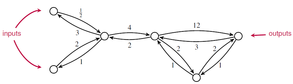
If the rate of 4 that describes the w2 to w1 transition was increased to a very large number, the coarse-grain solution would result in the w to y transition asymptotically converging to 9. This is a basic form of order-reduction for stiff problems.
https://en.wikipedia.org/wiki/Model_order_reduction
@John . By the way is Kenny reading the comments to this blog post?

OK thanks. Now I am more or less sure that I understand what you mean with the notation
As said I might have a different approach to derive a Hamiltonian from a diagram, but with the approach I sofar used, the Hamiltonian as derived with my approach would not be lumpable:
@Paul
I don’t see what this have to do with stiffness problems, but if 4 gets big then with the above hamiltonian the w to y transition would converge to 9 only for a specific section.
I doubt Kenny is reading the comments here. I’ll tell him about these comments.
Hi Nad,
The image in the tweet was taken from back when we were originally considering more general coarse-grainings of Markov processes. Later on, for category theoretic reasons, we decided to only work with Markov processes that were lumpable, since lumpability is precisely the condition needed for the Hamiltonian of the new Markov process to be independent of the choice of stochastic section s. As you noticed, the image in the tweet isn’t lumpable (at least not in the manner that is being visually suggested) since the rates of the edges going from both of the states w1 and w2 to the state y are not the same. They are in the example in the paper.
It’s also perhaps worth noting that the edge with rate 4 going from the state w2 to the state w1 plays no role in the lumped Markov process, which intuitively makes sense: anything in either of the states w1 or w2 will transition to state y at the same rate in the case where the original Markov process is lumpable, and transitioning between states w1 and w2 will not affect this.
Hello Kenny
thanks for replying. You wrote:
Frankly I have problems to see why this is a category theoretic question. In particular I haven’t sofar understood what this lumpability is needed for. I could have imagined e.g. that an internal lumpability might for example not change the relations between input and outputs of a Markov network, but I haven’t found a remark similar to that.
I searched the text for all occasions of the word “lump”, but apart from the reference it didn’t appear in the text after theorem 3.10.
Nad wrote:
It sounds like you’re talking about Lemma 5.3, which says that coarse-graining is compatible with black-boxing. You’ll note that the proof uses the equation
In our paper we define ‘lumpability’ in Definition 3.4. Theorem 3.10 gives 3 equivalent conditions for lumpability. The best one is condition (ii):
This is clearly equivalent to
This condition says that two things are the same:
1) evolving a state in time using our original Markov process with Hamiltonian and then coarse-graining it with
  ,
,
2) coarse-graining a state with and then evolving it in time using the coarse-grained Markov process with Hamiltonian
  .
.
Since this is so nice, we build the equation into the definition of ‘morphism between open Markov processes’ in Definition 3.4. In the rest of the paper we study these morphisms and never mention the word ‘lump’.
We need the condition to prove most of the interesting results in the paper. For example, Lemma 5.3.
The literature on Markov processes talks about lumpability, but they usually use the equivalent condition (iii) as their definition of lumpability.
John wrote:
Well, as said I was looking for a remark like that, but I didn’t and unfortunately still don’t see that “coarse-graining is compatible with black-boxing” is explained in Lemma 5.3:
That is even if you tell me that “build the equation into the definition of ‘morphism between open Markov processes” I don’t see why Lemma 5.3. says “coarse-graining is compatible with black-boxing” and in particular what you mean with “compatible.” This seems to be hidden in those cryptic diagrams. But anyways I got now a rough idea of what you were doing here.
Thanks for being so publicly confused about our paper; having worked on it for a year the meaning of the formalism has become obvious to Kenny and me, but you’re reminding me that a few sentences here and there could help explain its meaning.
Lemma 5.3 is about what happens when we apply the 2-functor , which is black-boxing, to 2-morphisms in Mark, which are morphisms between open Markov processes. The simplest morphisms between open Markov processes are coarse-grainings. So, the Lemma says what happens when we black-box a coarse-graining.
The simplest case is when the maps and
and  in the diagram are identity functions. This means that we’re leaving the input and output states alone. In this case, Lemma 5.3 says that the relation between input and output probabilities and flows in steady state are the same for the original open Markov process and the coarse-grained open Markov process.
I thought that might be what you were trying to say here:
This is true if by “the relations between inputs and outputs” you mean “the relation between input and output probabilities and flows in steady state”. This relation is what black-boxing gives us.
The double category formalism, with its supposedly cryptic diagrams, is just a way of drawing open Markov processes and the morphisms between them, e.g. coarse-grainings. With this style of picture, the coarse-grainings look like rectangles. The basic operations on coarse-grainings look like ways of sticking together rectangles to get bigger rectangles. The rules these operations obey turn into intuitive rules about sticking together rectangles.
That’s the whole point of double categories. Double categories are “the algebra of rectangles”, just as categories are “the algebra of arrows”.
We don’t explain this, because this paper was written for people who are comfortable with double categories. Explaining double categories would double the length of this paper.
I said morphisms between open Markov processes look like rectangles. But the simplest morphisms between open Markov processes are coarse-grainings, so let me talk just about coarse-grainings. The two main operations on these are:
1) We can compose coarse-grainings of open Markov processes “horizontally” by attaching the outputs of one to the inputs of another.
2) We can compose coarse-grainings of open Markov processes “vertically” by doing first one and then another: coarse-graining and then coarse-graining some more.
We can stick together two rectangles either horizontally or vertically, and that’s how we draw operations 1) and 2). Some nontrivial laws governing these operations then drawn as obvious-looking laws about sticking rectangles together.
Double categories were introduced in the 1960s by Charles Ehresmann. More recently they have found their way into applied mathematics. They been used to study various things, including open dynamical systems:
• Eugene Lerman and David Spivak, An algebra of open continuous time dynamical systems and networks.
open electrical circuits and chemical reaction networks:
• Kenny Courser, A bicategory of decorated cospans, Theory and Applications of Categories 32 (2017), 995–1027.
open discrete-time Markov chains:
• Florence Clerc, Harrison Humphrey and P. Panangaden, Bicategories of Markov processes, in Models, Algorithms, Logics and Tools, Lecture Notes in Computer Science 10460, Springer, Berlin, 2017, pp. 112–124.
and coarse-graining for open continuous-time Markov chains:
• John Baez and Kenny Courser, Coarse-graining open Markov processes. (Blog article here.)
As noted by Shulman, the easiest way to get a symmetric monoidal bicategory is often to first construct a symmetric monoidal double category:
• Mike Shulman, Constructing symmetric monoidal bicategories.
I’m giving a talk on work I did with Kenny Courser. It’s part of the ACT2020 conference, and it’s happening on 20:40 UTC on Tuesday July 7th, 2020. (That’s 1:40 pm here in California, just so I don’t forget.)
Like all talks at this conference, you can watch it live on Zoom or on YouTube. It’ll also be recorded, so you can watch it later on YouTube too, somewhere here.
You can see my slides now, and read some other helpful things:
• Coarse-graining open Markov processes.
My student Kenny Courser‘s thesis has hit the arXiv:
• Kenny Courser, Open Systems: A Double Categorical Perspective, Ph.D. thesis, U. C. Riverside, 2020.