The Maxwell relations are equations that show up whenever we have a smooth convex function

They say that the mixed partial derivatives of 
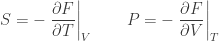
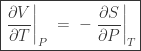
For example, here is one of the Maxwell relations that people often use when studying a thermodynamic system like a cylinder of gas or a beaker of liquid:
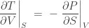
where:
• 
• 
• 
• 
There are also three more Maxwell relations involving these quantities. They all have the same general look, though half contain minus signs and half don’t. So, they’re quite tiresome to memorize. It’s more interesting to figure out what’s really going on here!
I already gave one story about what’s going on: we start with a function

we get the Maxwell relation I wrote above, simply by using the standard definitions of 


Let me show you in detail how this works, but without explaining why I’m choosing the particular ‘bunch of other functions’ that I’ll use. There is a way to explain that using the concept of Legendre transform. But next time I’ll give a very different approach to the Maxwell relations, based on this paper:
• David J. Ritchie, A simple method for deriving Maxwell’s relations, American Journal of Physics 36 (1958), 760–760.
This sidesteps the whole business of choosing a ‘bunch of other functions’, and I think it’s very nice.
What follows is a bit mind-numbing, so let me tell you what to pay attention to. I’ll do the same general sort of calculation four times, first starting with any convex smooth function 
The first relation
We start with any smooth convex function 

This says
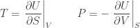
These are the usual definitions of the temperature 
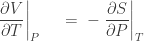
The commuting of mixed partials implies
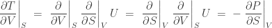
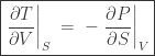
giving the first of the Maxwell relations:
The second relation
Next, let’s define the Helmholtz free energy

Taking its differential we get

so if we think of 

The commuting of mixed partials implies
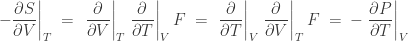
giving the second of the Maxwell relations:

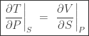
The third relation
Copying what we did to get the second relation, let’s define the enthalpy

Taking its differential we get

so if we think of 


The commuting of mixed partials implies

giving the third of the Maxwell relations:
The fourth relation
Combining the last two tricks, let’s define the Gibbs free energy

Taking its differential we get

so if we think of 


The commuting of mixed partials implies
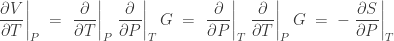
giving the fourth and final Maxwell relation:
Conclusions
I hope you’re a bit unsatisfied, for two main reasons.
The first question you should have is this: why did we chose these four functions to work with:

The pattern of signs is not really significant here: if we hadn’t followed tradition and stuck a minus sign in our definition of
everything would look more systematic, and we’d use these four functions:

This would make it easier to guess how everything works if instead of a function 

and define a bunch of functions

called ‘conjugate quantities’.
Then, we could get 


Then we could take mixed partial derivatives of these functions, note that the mixed partial derivatives commute, and get a bunch of Maxwell relations — maybe

of them! (Sanity check: when 
The second question you should have is: how did I sneakily switch from thinking of 
Answering these questions well might get us into a bit of contact geometry. That would be nice. But instead of answering these questions next time, I’ll talk about Ritchie’s approach to deriving Maxwell’s equations, which seems to sidestep the two questions I just raised!
Just for fun
Finally: students of thermodynamics are often forced to memorize the Maxwell relations. They sometimes use the thermodynamic square:

where for some idiotic reason the 
If you like puzzles, maybe you can figure out how the thermodynamic square works if you stare at it along with the four Maxwell equations I derived:


Again, it probably be easier if we hadn’t stuck a minus sign into the definition of pressure. If you get stuck, click on the link.
Unfortunately the thermodynamic square is itself so hard to memorize that students resort to a mnemonic for that! Sometimes they say “Good Physicists Have Studied Under Very Fine Teachers” which gives the letters “GPHSUVFT” that you see as you go around the square.
I will never try to remember any of these mnemonics. But I wonder if there’s something deeper going on here. So:
Puzzle. How does the thermodynamic square generalize if
• Part 1: a proof of Maxwell’s relations using commuting partial derivatives.
• Part 2: a proof of Maxwell’s relations using 2-forms.
• Part 3: the physical meaning of Maxwell’s relations, and their formulation in terms of symplectic geometry.
For how Maxwell’s relations are connected to Hamilton’s equations, see this post:


What’s the technical term for negative pressure? Suction?
I don’t know if there is an official technical term. Maybe it’s “tension”.
If the cosmological constant works the way we think, empty space has a slight negative pressure. People call it “dark energy” but some physicists think “invisible tension” would be more accurate. Or you could just say the universe sucks.
I usually see ‘tension’ measured in units of force. There's ‘tensile stress’ or ‘tensile strength’, measured in units of pressure, but this is usually not a simple measure of negative pressure but the maximum amount of negative pressure that an object can withstand before being torn apart.
Copied from my comment on part 2:
Of course, not all situations involve simple hydrostatic pressure; some require a full stress tensor and instead of one has something like
  (where hydrostatic pressure is the special case
  ). Notation tends to vary between linear elasticity theory, fluid dynamics, and other fields where the stress and deformation tensors appear.
Yes, in Parts 1 and 2 I study Maxwell’s relations for any smooth function of 2 variables
(I call this function but it can be anything.) Then in Part 3 I jump from the 2-variable case to the n-variable case. With a bit more sophisticated math we could study the case of
where is an infinite-dimensional vector space or infinite-dimensional manifold. The key ideas are very general.
To get from to the other potentials one need not know about the potentials in advance but rather simply extract complete differentials (exact 1-forms) from the right-hand side. For example, to get
  one extracts
  , i.e. we write
  as
as  and move the term
  to the left-hand side to get the complete differential
  . Extracting
  separately or together with
  lead to the other two potentials.
Thanks. Yes, one can find the potentials this way. In this series of posts I was heading toward a proof of Maxwell’s relations that doesn’t involve these potentials, so I was emphasizing—a bit unfairly—how annoying they can be. But they are interesting and important in their own right, along with the theory of Legendre transforms.
I can only say: It is a wonderful post, just like the 2 other in this series! Congratulations John! Your legacy as blogger, teacher of mathematics, and other stuff is going to last forever (if a meteorite or catastrophe don’t annihilate our world! I’m beginning to think that the solution to the Fermi paradox is that intelligent species has really a short time to develop interstellar skills but I can be wrong! The Great Filter is upon us!)
Thanks! I don’t think anything lasts forever—it’s strange how we wish things would.
Well, obviously as a physicist myself I would say…At least longer than the lifetime of the proton! and a generalized thermodynamics using 3-forms or n-forms. Another issue I wondered in those times was if there is any other form of thermodynamics possible (now I know the answer is yes, as there is Tsallis, Renyi and other types of thermostatistics!). Do you know if there is any about that? Blender and Nevir just formulated fluid dynamics using a Nambu form. And I think another guy even formulated electromagnetism as a Nambu-type fluid! I google it and checked it in my database of articles: https://www.academia.edu/37174521/Nambu_brackets_for_the_electromagnetic_field Worth reading yet! If any reader knows about any other n-ary works about fluid thermodynamics or alike I would be pleased to read them all.
By the way, do you think a 3-variable or n-variable Poisson-like variant (maybe Nambu mechanics) could be possible? As an undergraduated, when reading about Nambu mechanics in the library, I wondered if someone had considered something like
The intuitive argument in favor of Nambu-like dynamics is the presence of a chemical potentiatl and other charges/potentials in the first principle, e.g.:
 or
or  . Then, one would expect something like
 and its dual form
  to be invariant forms similar to the 2-form in common thermodynamics. What do you think?
In the simple case considered in this article, we don't have or
or  ; we have
  and
and  (added together with a minus sign). So this just looks like moving from
  variables to
  variables but still with a
  -form:
  .
.
Yes Tony, I realized I wrote the WRONG variable in the 2-form, but I can not edit my posts here :(. My mistake…
With respect to n-ary Thermodynamics I was watching some papers yesterday about geometric thermodynamics in black holes and/or fluid dynamics in which there are some Nambu formulations! However, I am not sure I understand the formulation of Nambu dynamics and the fundamental identity when quantized. If my memory doesn’t fail, there are some algebras by Filipov (or a guy with similar name) which studied n-ary algebras in Nambu-like style, but I have not read Nambu dynamics papers for a while. Perhaps, it’s time to read about Nambu mechanics again. Even more, I found out that there is a dissipative version of classical mechanics combining the metric and a Poisson bracket structure, something called metriplectic dynamics. I am not sure of what is the capability of that mechanics but I will also reseach on it…
When we go to more variables in thermodynamics we still get a cotangent bundle equipped with the usual 2-form, which is a symplectic structure, and the submanifold of thermodynamic states is a Lagrangian submanifold. This is sort of ‘well-known’, though people often phrase the idea using contact geometry instead of symplectic geometry, and it’s not incredibly easy to find a clear account of all this. You can read a tiny bit more about near the very end here:
• Classical mechanics versus thermodynamics.
where I discuss the case where we keep track of particle number (for just one kind of particle) and the chemical potential. Near the end here:
• Maxwell’s relations (part 3).
I describe the math in the general case, but not specific examples from thermodynamics.
Then, what should be the motivation for a Nambu formulation of (generalized) thermodynamics, if any, as some research papers about black holes do indeed? Further symmetries?
I’ve never understood Nambu mechanics.
Maxwell Relations are commonly known as a set of four partial differential equations between four thermodynamic quantities or potentials: pressure (P), volume (V), temperature (T), and entropy (S).
[….]