Tutorial on Categorical Semantics of Entropy

Here are two talks on the categorical semantics of entropy, given on Wednesday May 11th 2022 at CUNY. First one there’s one by me and then starting around 1:31:00 there’s one by Tai-Danae Bradley:

My talk is called “Shannon entropy from category theory”:

Shannon entropy is a powerful concept. But what properties single out Shannon entropy as special? Instead of focusing on the entropy of a probability measure on a finite set, it can help to focus on the “information loss”, or change in entropy, associated with a measure-preserving function. Shannon entropy then gives the only concept of information loss that is functorial, convex-linear and continuous. This is joint work with Tom Leinster and Tobias Fritz.

Tai-Danae Bradley’s is called “Operads and entropy”:

This talk will open with a basic introduction to operads and their representations, with the main example being the operad of probabilities. I’ll then give a light sketch of how this framework leads to a small, but interesting, connection between information theory, abstract algebra, and topology, namely a correspondence between Shannon entropy and derivations of the operad of probabilities.

My talk is mainly about this paper:

• John Baez, Tobias Fritz and Tom Leinster, A characterization of entropy in terms of information loss, 2011.

and hers is mainly about this:

• Tai-Danae Bradley, Entropy as a topological operad derivation, 2021.

Here are some related readings:

• Tom Leinster, An operadic introduction to entropy, 2011.

• John Baez and Tobias Fritz, A Bayesian characterization of relative entropy, 2014.

• Tom Leinster, A short characterization of relative entropy, 2017.

• Nicolas Gagné and Prakash Panangaden,
A categorical characterization of relative entropy on standard Borel spaces, 2017.

• Tom Leinster, Entropy and Diversity: the Axiomatic Approach, 2020.

• Arthur Parzygnat, A functorial characterization of von Neumann entropy, 2020.

• Arthur Parzygnat, Towards a functorial description of quantum relative entropy, 2021.

Shannon Entropy from Category Theory

I’m giving a talk at Categorical Semantics of Entropy on Wednesday May 11th, 2022. You can watch it live on Zoom if you register, or recorded later. Here’s the idea:

Shannon entropy is a powerful concept. But what properties single out Shannon entropy as special? Instead of focusing on the entropy of a probability measure on a finite set, it can help to focus on the “information loss”, or change in entropy, associated with a measure-preserving function. Shannon entropy then gives the only concept of information loss that is functorial, convex-linear and continuous. This is joint work with Tom Leinster and Tobias Fritz.

You can see the slides now, here. I talk a bit about all these papers:

• John Baez, Tobias Fritz and Tom Leinster, A characterization of entropy in terms of information loss, 2011.

• Tom Leinster, An operadic introduction to entropy, 2011.

• John Baez and Tobias Fritz, A Bayesian characterization of relative entropy, 2014.

• Tom Leinster, A short characterization of relative entropy, 2017.

• Nicolas Gagné and Prakash Panangaden, A categorical characterization of relative entropy on standard Borel spaces, 2017.

• Tom Leinster, Entropy and Diversity: the Axiomatic Approach, 2020.

• Arthur Parzygnat, A functorial characterization of von Neumann entropy, 2020.

• Arthur Parzygnat, Towards a functorial description of quantum relative entropy, 2021.

• Tai-Danae Bradley, Entropy as a topological operad derivation, 2021.

Categorical Semantics of Entropy

There will be a workshop on the categorical semantics of entropy at the CUNY Grad Center in Manhattan on Friday May 13th, organized by John Terilla. I was kindly invited to give an online tutorial beforehand on May 11, which I will give remotely to save carbon. Tai-Danae Bradley will also be giving a tutorial that day in person:

• Tutorial: Categorical Semantics of Entropy, Wednesday 11 May 2022, 13:00–16:30 Eastern Time, Room 5209 at the CUNY Graduate Center and via Zoom. Organized by John Terilla. To attend, register here.

12:00-1:00 Eastern Daylight Time — Lunch in Room 5209.

1:00-2:30 — Shannon entropy from category theory, John Baez, University of California Riverside; Centre for Quantum Technologies (Singapore); Topos Institute.

Shannon entropy is a powerful concept. But what properties single out Shannon entropy as special? Instead of focusing on the entropy of a probability measure on a finite set, it can help to focus on the “information loss”, or change in entropy, associated with a measure-preserving function. Shannon entropy then gives the only concept of information loss that is functorial, convex-linear and continuous. This is joint work with Tom Leinster and Tobias Fritz.

2:30-3:00 — Coffee break.

3:00-4:30 — Operads and entropy, Tai-Danae Bradley, The Master’s University; Sandbox AQ.

This talk will open with a basic introduction to operads and their representations, with the main example being the operad of probabilities. I’ll then give a light sketch of how this framework leads to a small, but interesting, connection between information theory, abstract algebra, and topology, namely a correspondence between Shannon entropy and derivations of the operad of probabilities.

• Symposium on Categorical Semantics of Entropy, Friday 13 May 2022, 9:30-3:15 Eastern Daylight Time, Room 5209 at the CUNY Graduate Center and via Zoom. Organized by John Terilla. To attend, register here.

9:30-10:00 Eastern Daylight Time — Coffee and pastries in Room 5209.

10:00-10:45 — Operadic composition of thermodynamic systems, Owen Lynch, Utrecht University.

The maximum entropy principle is a fascinating and productive lens with which to view both thermodynamics and statistical mechanics. In this talk, we present a categorification of the maximum entropy principle, using convex spaces and operads. Along the way, we will discuss a variety of examples of the maximum entropy principle and show how each application can be captured using our framework. This approach shines a new light on old constructions. For instance, we will show how we can derive the canonical ensemble by attaching a probabilistic system to a heat bath. Finally, our approach to this categorification has applications beyond the maximum entropy principle, and we will give an hint of how to adapt this categorification to the formalization of the composition of other systems.

11:00-11:45 — Polynomial functors and Shannon entropy, David Spivak, MIT and the Topos Institute.

The category Poly of polynomial functors in one variable is extremely rich, brimming with categorical gadgets (e.g. eight monoidal products, two closures, limits, colimits, etc.) and applications including dynamical systems, databases, open games, and cellular automata. In this talk I’ll show that objects in Poly can be understood as empirical distributions. In part using the standard derivative of polynomials, we obtain a functor to Set × Set^op which encodes an invariant of a distribution as a pair of sets. This invariant is well-behaved in the sense that it is a distributive monoidal functor: it acts on both distributions and maps between them, and it preserves both the sum and the tensor product of distributions. The Shannon entropy of the original distribution is then calculated directly from the invariant, i.e. only in terms of the cardinalities of these two sets. Given the many applications of polynomial functors and of Shannon entropy, having this link between them has potential to create useful synergies, e.g. to notions of entropic causality or entropic learning in dynamical systems.

12:00-1:30 — Lunch in Room 5209

1:30-2:15 — Higher entropy, Tom Mainiero, Rutgers New High Energy Theory Center.

Is the frowzy state of your desk no longer as thrilling as it once was? Are numerical measures of information no longer able to satisfy your needs? There is a cure! In this talk we’ll learn about: the secret topological lives of multipartite measures and quantum states; how a homological probe of this geometry reveals correlated random variables; the sly decategorified involvement of Shannon, Tsallis, Réyni, and von Neumann in this larger geometric conspiracy; and the story of how Gelfand, Neumark, and Segal’s construction of von Neumann algebra representations can help us uncover this informatic ruse. So come to this talk, spice up your entropic life, and bring new meaning to your relationship with disarray.

2:30-3:15 — On characterizing classical and quantum entropy, Arthur Parzygnat, Institut des Hautes Études Scientifiques.

In 2011, Baez, Fritz, and Leinster proved that the Shannon entropy can be characterized as a functor by a few simple postulates. In 2014, Baez and Fritz extended this theorem to provide a Bayesian characterization of the classical relative entropy, also known as the Kullback–Leibler divergence. In 2017, Gagné and Panangaden extended the latter result to include standard Borel spaces. In 2020, I generalized the first result on Shannon entropy so that it includes the von Neumann (quantum) entropy. In 2021, I provided partial results indicating that the Umegaki relative entropy may also have a Bayesian characterization. My results in the quantum setting are special applications of the recent theory of quantum Bayesian inference, which is a non-commutative extension of classical Bayesian statistics based on category theory. In this talk, I will give an overview of these developments and their possible applications in quantum information theory.

Wine and cheese reception to follow, Room 5209.

Information Geometry (Part 21)

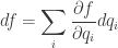
Last time I ended with a formula for the ‘Gibbs distribution’: the probability distribution that maximizes entropy subject to constraints on the expected values of some observables.

This formula is well-known, but I’d like to derive it here. My argument won’t be up to the highest standards of rigor: I’ll do a bunch of computations, and it would take more work to state conditions under which these computations are justified. But even a nonrigorous approach is worthwhile, since the computations will give us more than the mere formula for the Gibbs distribution.

I’ll start by reminding you of what I claimed last time. I’ll state it in a way that removes all unnecessary distractions, so go back to Part 20 if you want more explanation.

The Gibbs distribution

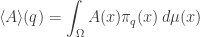
Take a measure space with measure Suppose there is a probability distribution on that maximizes the entropy

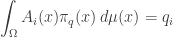
subject to the requirement that some integrable functions on have expected values equal to some chosen list of numbers

(Unlike last time, now I’m writing and with superscripts rather than subscripts, because I’ll be using the Einstein summation convention: I’ll sum over any repeated index that appears once as a a superscript and once as a subscript.)

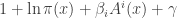
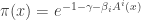
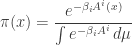
Furthermore, suppose depends smoothly on I’ll call it to indicate its dependence on Then, I claim is the so-called Gibbs distribution

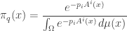
where

and

is the entropy of

Let’s show this is true!

Finding the Gibbs distribution

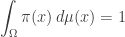
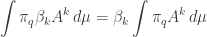
So, we are trying to find a probability distribution that maximizes entropy subject to these constraints:

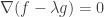
We can solve this problem using Lagrange multipliers. We need one Lagrange multiplier, say for each of the above constraints. But it’s easiest if we start by letting range over all of that is, the space of all integrable functions on Then, because we want to be a probability distribution, we need to impose one extra constraint

To do this we need an extra Lagrange multiplier, say

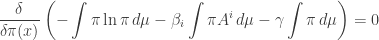
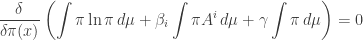
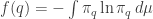
So, that’s what we’ll do! We’ll look for critical points of this function on

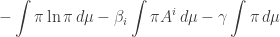
Here I’m using some tricks to keep things short. First, I’m dropping the dummy variable x which appeared in all of the integrals we had: I’m leaving it implicit. Second, all my integrals are over so I won’t say that. And third, I’m using the Einstein summation convention, so there’s a sum over i implicit here.

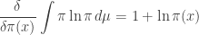
Okay, now let’s do the variational derivative required to find a critical point of this function. When I was a math major taking physics classes, the way physicists did variational derivatives seemed like black magic to me. Then I spent months reading how mathematicians rigorously justified these techniques. I don’t feel like a massive digression into this right now, so I’ll just do the calculations—and if they seem like black magic, I’m sorry!

We need to find obeying

or in other words

First we need to simplify this expression. The only part that takes any work, if you know how to do variational derivatives, is the first term. Since the derivative of is we have

The second and third terms are easy, so we get

       

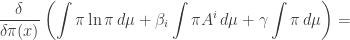
Thus, we need to solve this equation:

That’s easy to do:

Good! It’s starting to look like the Gibbs distribution!

We now need to choose the Lagrange multipliers and to make the constraints hold. To satisfy this constraint

we must choose so that

or in other words

Plugging this into our earlier formula

we get this:

Great! Even more like the Gibbs distribution!

By the way, you must have noticed the “1” that showed up here:

It buzzed around like an annoying fly in the otherwise beautiful calculation, but eventually went away. This is the same irksome “1” that showed up in Part 19. Someday I’d like to say a bit more about it.

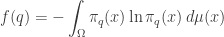
Now, where were we? We were trying to show that

minimizes entropy subject to our constraints. So far we’ve shown

is a critical point. It’s clear that

so really is a probability distribution. We should show it actually maximizes entropy subject to our constraints, but I will skip that. Given that, will be our claimed Gibbs distribution if we can show

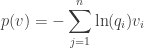
This is interesting! It’s saying our Lagrange multipliers actually equal the so-called conjugate variables given by

where is the entropy of

There are two ways to show this: the easy way and the hard way. The easy way is to reflect on the meaning of Lagrange multipliers, and I’ll sketch that way first. The hard way is to use brute force: just compute and show it equals This is a good test of our computational muscle—but more importantly, it will help us discover some interesting facts about the Gibbs distribution.

The easy way

Consider a simple Lagrange multiplier problem where you’re trying to find a critical point of a smooth function

subject to the constraint

for some smooth function

and constant c. (The function f here has nothing to do with the f in the previous sections.) To answer this we introduce a Lagrange multiplier and seek points where

This works because the above equation says

Geometrically this means we’re at a point where the gradient of points at right angles to the level surface of

Thus, to first order we can’t change by moving along the level surface of

But also, if we start at a point where

and we begin moving in any direction, the function will change at a rate equal to times the rate of change of . That’s just what the equation says! And this fact gives a conceptual meaning to the Lagrange multiplier

Our situation is more complicated, since our functions are defined on the infinite-dimensional space and we have an n-tuple of constraints with an n-tuple of Lagrange multipliers. But the same principle holds.

So, when we are at a solution of our constrained entropy-maximization problem, and we start moving the point by changing the value of the ith constraint, namely the rate at which the entropy changes will be times the rate of change of So, we have

But this is just what we needed to show!

The hard way

Here’s another way to show

We start by solving our constrained entropy-maximization problem using Lagrange multipliers. As already shown, we get

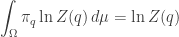
Then we’ll compute the entropy

Then we’ll differentiate this with respect to and show we get

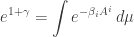
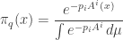
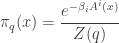
Let’s try it! The calculation is a bit heavy, so let’s write for the so-called partition function

so that

and the entropy is

This is the sum of two terms. The first term

is times the expected value of with respect to the probability distribution all summed over But the expected value of is so we get

The second term is easier:

since integrates to 1 and the partition function doesn’t depend on

Putting together these two terms we get an interesting formula for the entropy:

This formula is one reason this brute-force approach is actually worthwhile! I’ll say more about it later.

But for now, let’s use this formula to show what we’re trying to show, namely

For starters,

where we played a little Kronecker delta game with the second term.

Now we just need to compute the third term:

Ah, you don’t know how good it feels, after years of category theory, to be doing calculations like this again!

Now we can finish the job we started:

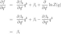
Voilà!

Conclusions

We’ve learned the formula for the probability distribution that maximizes entropy subject to some constraints on the expected values of observables. But more importantly, we’ve seen that the anonymous Lagrange multipliers that show up in this problem are actually the partial derivatives of entropy! They equal

Thus, they are rich in meaning. From what we’ve seen earlier, they are ‘surprisals’. They are analogous to momentum in classical mechanics and have the meaning of intensive variables in thermodynamics:

	Classical Mechanics	Thermodynamics	Probability Theory
q	position	extensive variables	probabilities
p	momentum	intensive variables	surprisals
S	action	entropy	Shannon entropy

Furthermore, by showing the hard way we discovered an interesting fact. There’s a relation between the entropy and the logarithm of the partition function:

(We proved this formula with replacing but now we know those are equal.)

This formula suggests that the logarithm of the partition function is important—and it is! It’s closely related to the concept of free energy—even though ‘energy’, free or otherwise, doesn’t show up at the level of generality we’re working at now.

This formula should also remind you of the tautological 1-form on the cotangent bundle namely

It should remind you even more of the contact 1-form on the contact manifold namely

Here is a coordinate on the contact manifold that’s a kind of abstract stand-in for our entropy function

So, it’s clear there’s a lot more to say: we’re seeing hints of things here and there, but not yet the full picture.

---

For all my old posts on information geometry, go here:

• Information geometry.

Information Geometry (Part 20)

Last time we worked out an analogy between classical mechanics, thermodynamics and probability theory. The latter two look suspiciously similar:

	Classical Mechanics	Thermodynamics	Probability Theory
q	position	extensive variables	probabilities
p	momentum	intensive variables	surprisals
S	action	entropy	Shannon entropy

This is no coincidence. After all, in the subject of statistical mechanics we explain classical thermodynamics using probability theory—and entropy is revealed to be Shannon entropy (or its quantum analogue).

Now I want to make this precise.

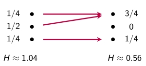
To connect classical thermodynamics to probability theory, I’ll start by discussing ‘statistical manifolds’. I introduced the idea of a statistical manifold in Part 7: it’s a manifold equipped with a map sending each point to a probability distribution on some measure space Now I’ll say how these fit into the second column of the above chart.

Then I’ll talk about statistical manifolds of a special sort used in thermodynamics, which I’ll call ‘Gibbsian’, since they really go back to Josiah Willard Gibbs.

In a Gibbsian statistical manifold, for each the probability distribution is a ‘Gibbs distribution’. Physically, these Gibbs distributions describe thermodynamic equilibria. For example, if you specify the volume, energy and number of particles in a box of gas, there will be a Gibbs distribution describing what the particles do in thermodynamic equilibrium under these conditions. Mathematically, Gibbs distributions maximize entropy subject to some constraints specified by the point

More precisely: in a Gibbsian statistical manifold we have a list of observables whose expected values serve as coordinates for points and is the probability distribution that maximizes entropy subject to the constraint that the expected value of is We can derive most of the interesting formulas of thermodynamics starting from this!

Statistical manifolds

Let’s fix a measure space with measure A statistical manifold is then a manifold equipped with a smooth map assigning to each point a probability distribution on which I’ll call So, is a function on with

and

for all

The idea here is that the space of all probability distributions on may be too huge to understand in as much detail as we’d like, so instead we describe some of these probability distributions—a family parametrized by points of some manifold —using the map This is the basic idea behind parametric statistics.

Information geometry is the geometry of statistical manifolds. Any statistical manifold comes with a bunch of interesting geometrical structures. One is the ‘Fisher information metric’, a Riemannian metric I explained in Part 7. Another is a 1-parameter family of connections on the tangent bundle which is important in Amari’s approach to information geometry. You can read about this here:

• Hiroshi Matsuzoe, Statistical manifolds and affine differential geometry, in Advanced Studies in Pure Mathematics 57, pp. 303–321.

I don’t want to talk about it now—I just wanted to reassure you that I’m not completely ignorant of it!

I want to focus on the story I’ve been telling, which is about entropy. Our statistical manifold comes with a smooth entropy function

namely

We can use this entropy function to do many of the things we usually do in thermodynamics! For example, at any point where this function is differentiable, its differential gives a cotangent vector

which has an important physical meaning. In coordinates we have

and we call the intensive variable conjugate to For example if is energy, will be ‘coolness’: the reciprocal of temperature.

Defining this way gives a Lagrangian submanifold

of the cotangent bundle We can also get contact geometry into the game by defining a contact manifold and a Legendrian submanifold

But I’ve been talking about these ideas for the last three episodes, so I won’t say more just now! Instead, I want to throw a new idea into the pot.

Gibbsian statistical manifolds

Thermodynamics, and statistical mechanics, spend a lot of time dealing with statistical manifold of a special sort I’ll call ‘Gibbsian’. In these, each probability distribution is a ‘Gibbs distribution’, meaning that it maximizes entropy subject to certain constraints specified by the point

How does this work? For starters, an integrable function

is called a random variable, or in physics an observable. The expected value of an observable is a smooth real-valued function on our statistical manifold

given by

In other words, is a function whose value at at any point is the expected value of with respect to the probability distribution

Now, suppose our statistical manifold is n-dimensional and we have n observables Their expected values will be smooth functions on our manifold—and sometimes these functions will be a coordinate system!

This may sound rather unlikely, but it’s really not so outlandish. Indeed, if there’s a point such that the differentials of the functions are linearly independent at this point, these functions will be a coordinate system in some neighborhood of this point, by the inverse function theorem. So, we can take this neighborhood, use it as our statistical manifold, and the functions will be coordinates.

So, let’s assume the expected values of our observables give a coordinate system on Let’s call these coordinates so that

Now for the kicker: we say our statistical manifold is Gibbsian if for each point is the probability distribution that maximizes entropy subject to the above condition!

Which condition? The condition saying that

for all i. This is just the previous equation spelled out so that you can see it’s a condition on

This assumption of the entropy-maximizing nature of is a very powerful, because it implies a useful and nontrivial formula for It’s called the Gibbs distribution:

for all

Here is the intensive variable conjugate to while is the partition function: the thing we must divide by to make sure integrates to 1. In other words:

By the way, this formula may look confusing at first, since the left side depends on the point in our statistical manifold, while there’s no visible in the right side! Do you see what’s going on?

I’ll tell you: the conjugate variable sitting on the right side of the above formula, depends on Remember, we got it by taking the partial derivative of the entropy in the direction

and the evaluating this derivative at the point

But wait a minute! here is the entropy—but the entropy of what?

The entropy of of course!

So there’s something circular about our formula for To know you need to know the conjugate variables but to compute these you need to know the entropy of

This is actually okay. While circular, the formula for is still true. It’s harder to work with than you might hope. But it’s still extremely useful.

Next time I’ll prove that this formula for is true, and do a few things with it. All this material was discovered by Gibbs in the late 1800’s, and it’s lurking any good book on statistical mechanics—but not phrased in the language of statistical manifolds. The physics textbooks usually consider special cases, like a box of gas where:

• is energy, is 1/temperature.

• is volume, is –pressure/temperature.

• is the number of particles, is chemical potential / pressure.

While these special cases are important and interesting, I’d rather be general!

Technical comments

I said “Any statistical manifold comes with a bunch of interesting geometrical structures”, but in fact some conditions are required. For example, the Fisher information metric is only well-defined and nondegenerate under some conditions on the map For example, if maps every point of to the same probability distribution, the Fisher information metric will vanish.

Similarly, the entropy function is only smooth under some conditions on

Furthermore, the integral

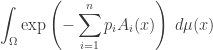
may not converge for all values of the numbers But in my discussion of Gibbsian statistical manifolds, I was assuming that an entropy-maximizing probability distribution with

actually exists. In this case the probability distribution is also unique (almost everywhere).

---

For all my old posts on information geometry, go here:

• Information geometry.

Information Geometry (Part 19)

Last time I figured out the analogue of momentum in probability theory, but I didn’t say what it’s called. Now I will tell you—thanks to some help from Abel Jansma and Toby Bartels.

SURPRISE: it’s called SURPRISAL!

This is a well-known concept in information theory. It’s also called ‘information content‘.

Let’s see why. First, let’s remember the setup. We have a manifold

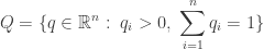
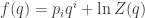
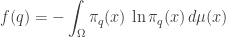
whose points are nowhere vanishing probability distributions on the set We have a function

called the Shannon entropy, defined by

For each point we define a cotangent vector by

As mentioned last time, this is the analogue of momentum in probability theory. In the second half of this post I’ll say more about exactly why. But first let’s compute it and see what it actually equals!

Let’s start with a naive calculation, acting as if the probabilities were a coordinate system on the manifold We get

so using the definition of the Shannon entropy we have

Now, the quantity is called the surprisal of the probability distribution at Intuitively, it’s a measure of how surprised you should be if an event of probability occurs. For example, if you flip a fair coin and it lands heads up, your surprisal is ln 2. If you flip 100 fair coins and they all land heads up, your surprisal is 100 times ln 2.

Of course ‘surprise’ is a psychological term, not a term from math or physics, so we shouldn’t take it too seriously here. We can derive the concept of surprisal from three axioms:

1. The surprisal of an event of probability is some function of , say
2. The less probable an event is, the larger its surprisal is:
3. The surprisal of two independent events is the sum of their surprisals:

It follows from work on Cauchy’s functional equation that must be of this form:

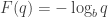
for some constant We shall choose the base of our logarithms, to be We had a similar freedom of choice in defining the Shannon entropy, and we will use base for both to be consistent. If we chose something else, it would change the surprisal and the Shannon entropy by the same constant factor.

So far, so good. But what about the irksome “-1” in our formula?

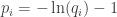
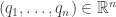
Luckily it turns out we can just get rid of this! The reason is that the probabilities are not really coordinates on the manifold They’re not independent: they must sum to 1. So, when we change them a little, the sum of their changes must vanish. Putting it more technically, the tangent space is not all of but just the subspace consisting of vectors whose components sum to zero:

The cotangent space is the dual of the tangent space. The dual of a subspace

is the quotient space

The cotangent space thus consists of linear functionals modulo those that vanish on vectors obeying the equation

Of course, we can identify the dual of with in the usual way, using the Euclidean inner product: a vector corresponds to the linear functional

From this, you can see that a linear functional vanishes on all vectors obeying the equation

if and only if its corresponding vector has

So, we get

In words: we can describe cotangent vectors to as lists of n numbers if we want, but we have to remember that adding the same constant to each number in the list doesn’t change the cotangent vector!

This suggests that our naive formula

is on the right track, but we’re free to get rid of the constant 1 if we want! And that’s true.

To check this rigorously, we need to show

for all We compute:

where in the second to last step we used our earlier calculation:

and in the last step we used

Back to the big picture

Now let’s take stock of where we are. We can fill in the question marks in the charts from last time, and combine those charts while we’re at it.

	Classical Mechanics	Thermodynamics	Probability Theory
q	position	extensive variables	probabilities
p	momentum	intensive variables	surprisals
S	action	entropy	Shannon entropy

What’s going on here? In classical mechanics, action is minimized (or at least the system finds a critical point of the action). In thermodynamics, entropy is maximized. In the maximum entropy approach to probability, Shannon entropy is maximized. This leads to a mathematical analogy that’s quite precise. For classical mechanics and thermodynamics, I explained it here:

• Classical mechanics versus thermodynamics (part 1).

• Classical mechanics versus thermodynamics (part 2).

These posts may give a more approachable introduction to what I’m doing now: now I’m bringing probability theory into the analogy, with a big emphasis on symplectic and contact geometry.

Let me spell out a bit of the analogy more carefully:

Classical Mechanics. In classical mechanics, we have a manifold whose points are positions of a particle. There’s an important function on this manifold: Hamilton’s principal function

What’s this? It’s basically action: is the action of the least-action path from the position at some earlier time to the position at time 0. The Hamilton–Jacobi equations say the particle’s momentum at time 0 is given by

Thermodynamics. In thermodynamics, we have a manifold whose points are equilibrium states of a system. The coordinates of a point are called extensive variables. There’s an important function on this manifold: the entropy

There is a cotangent vector at the point given by

The components of this vector are the intensive variables corresponding to the extensive variables.

Probability Theory. In probability theory, we have a manifold whose points are nowhere vanishing probability distributions on a finite set. The coordinates of a point are probabilities. There’s an important function on this manifold: the Shannon entropy

There is a cotangent vector at the point given by

The components of this vector are the surprisals corresponding to the probabilities.

In all three cases, is a symplectic manifold and imposing the constraint picks out a Lagrangian submanifold

There is also a contact manifold where the extra dimension comes with an extra coordinate that means

• action in classical mechanics,
• entropy in thermodynamics, and
• Shannon entropy in probability theory.

We can then decree that along with and these constraints pick out a Legendrian submanifold

There’s a lot more to do with these ideas, and I’ll continue next time.

---

For all my old posts on information geometry, go here:

• Information geometry.

Information Geometry (Part 18)

Last time I sketched how two related forms of geometry, symplectic and contact geometry, show up in thermodynamics. Today I want to explain how they show up in probability theory.

For some reason I haven’t seen much discussion of this! But people should have looked into this. After all, statistical mechanics explains thermodynamics in terms of probability theory, so if some mathematical structure shows up in thermodynamics it should appear in statistical mechanics… and thus ultimately in probability theory.

I just figured out how this works for symplectic and contact geometry.

Suppose a system has possible states. We’ll call these microstates, following the tradition in statistical mechanics. If you don’t know what ‘microstate’ means, don’t worry about it! But the rough idea is that if you have a macroscopic system like a rock, the precise details of what its atoms are doing are described by a microstate, and many different microstates could be indistinguishable unless you look very carefully.

We’ll call the microstates So, if you don’t want to think about physics, when I say microstate I’ll just mean an integer from 1 to n.

Next, a probability distribution assigns a real number to each microstate, and these numbers must sum to 1 and be nonnegative. So, we have though not every vector in is a probability distribution.

I’m sure you’re wondering why I’m using rather than to stand for an observable instead of a probability distribution. Am I just trying to confuse you?

No: I’m trying to set up an analogy to physics!

Last time I introduced symplectic geometry using classical mechanics. The most important example of a symplectic manifold is the cotangent bundle of a manifold A point of is a pair consisting of a point and a cotangent vector In classical mechanics the point describes the position of some physical system, while describes its momentum.

So, I’m going to set up an analogy like this:

	Classical Mechanics	Probability Theory
	position	probability distribution
	momentum	???

But what is to momentum as probability is to position?

A big clue is the appearance of symplectic geometry in thermodynamics, which I also outlined last time. We can use this to get some intuition about the analogue of momentum in probability theory.

In thermodynamics, a system has a manifold of states. (These are not the ‘microstates’ I mentioned before: we’ll see the relation later.) There is a function

describing the entropy of the system as a function of its state. There is a law of thermodynamics saying that

This equation picks out a submanifold of namely

Moreover this submanifold is Lagrangian: the symplectic structure vanishes when restricted to it:

This is very beautiful, but it goes by so fast you might almost miss it! So let’s clutter it up a bit with coordinates. We often use local coordinates on and describe a point using these coordinates, getting a point

They give rise to local coordinates on the cotangent bundle The are called extensive variables, because they are typically things that you can measure only by totalling up something over the whole system, like the energy or volume of a cylinder of gas. The are called intensive variables, because they are typically things that you can measure locally at any point, like temperature or pressure.

In these local coordinates, the symplectic structure on is the 2-form given by

The equation

serves as a law of physics that determines the intensive variables given the extensive ones when our system is in thermodynamic equilibrium. Written out using coordinates, this law says

It looks pretty bland here, but in fact it gives formulas for the temperature and pressure of a gas, and many other useful formulas in thermodynamics.

Now we are ready to see how all this plays out in probability theory! We’ll get an analogy like this, which goes hand-in-hand with our earlier one:

	Thermodynamics	Probability Theory
	extensive variables	probability distribution
	intensive variables	???

This analogy is clearer than the last, because statistical mechanics reveals that the extensive variables in thermodynamics are really just summaries of probability distributions on microstates. Furthermore, both thermodynamics and probability theory have a concept of entropy.

So, let’s take our manifold to consist of probability distributions on the set of microstates I was talking about before: the set Actually, let’s use nowhere vanishing probability distributions:

I’m requiring to ensure is a manifold, and also to make sure is differentiable: it ceases to be differentiable when one of the probabilities hits zero.

Since is a manifold, its cotangent bundle is a symplectic manifold And here’s the good news: we have a god-given entropy function

namely the Shannon entropy

So, everything I just described about thermodynamics works in the setting of plain old probability theory! Starting from our manifold and the entropy function, we get all the rest, leading up to the Lagrangian submanifold

that describes the relation between extensive and intensive variables.

For computations it helps to pick coordinates on Since the probabilities sum to 1, they aren’t independent coordinates on So, we can either pick all but one of them as coordinates, or learn how to deal with non-independent coordinates, which are already completely standard in projective geometry. Let’s do the former, just to keep things simple.

These coordinates on give rise in the usual way to coordinates and on the cotangent bundle These play the role of extensive and intensive variables, respectively, and it should be very interesting to impose the equation

where is the Shannon entropy. This picks out a Lagrangian submanifold

So, the question becomes: what does this mean? If this formula gives the analogue of momentum for probability theory, what does this analogue of momentum mean?

Here’s a preliminary answer: says how fast entropy increases as we increase the probability that our system is in the ith microstate. So if we think of nature as ‘wanting’ to maximize entropy, the quantity says how eager it is to increase the probability

Indeed, you can think of as a bit like pressure—one of the most famous intensive quantities in thermodynamics. A gas ‘wants’ to expand, and its pressure says precisely how eager it is to expand. Similarly, a probability distribution ‘wants’ to flatten out, to maximize entropy, and says how eager it is to increase the probability in order to do this.

But what can we do with this concept? And what does symplectic geometry do for probability theory?

I will start tackling these questions next time.

One thing I’ll show is that when we reduce thermodynamics to probability theory using the ideas of statistical mechanics, the appearance of symplectic geometry in thermodynamics follows from its appearance in probability theory.

Another thing I want to investigate is how other geometrical structures on the space of probability distributions, like the Fisher information metric, interact with the symplectic structure on its cotangent bundle. This will integrate symplectic geometry and information geometry.

I also want to bring contact geometry into the picture. It’s already easy to see from our work last time how this should go. We treat the entropy as an independent variable, and replace with a larger manifold having as an extra coordinate. This is a contact manifold with contact form

This contact manifold has a submanifold where we remember that entropy is a function of the probability distribution and define in terms of as usual:

And as we saw last time, is a Legendrian submanifold, meaning

But again, we want to understand what these ideas from contact geometry really do for probability theory!

---

For all my old posts on information geometry, go here:

• Information geometry.

Information Geometry (Part 17)

I’m getting back into information geometry, which is the geometry of the space of probability distributions, studied using tools from information theory. I’ve written a bunch about it already, which you can see here:

• Information geometry.

Now I’m fascinated by something new: how symplectic geometry and contact geometry show up in information geometry. But before I say anything about this, let me say a bit about how they show up in thermodynamics. This is more widely discussed, and it’s a good starting point.

Symplectic geometry was born as the geometry of phase space in classical mechanics: that is, the space of possible positions and momenta of a classical system. The simplest example of a symplectic manifold is the vector space with n position coordinates and n momentum coordinates

It turns out that symplectic manifolds are always even-dimensional, because we can always cover them with coordinate charts that look like When we change coordinates, it turns out that the splitting of coordinates into positions and momenta is somewhat arbitrary. For example, the position of a rock on a spring now may determine its momentum a while later, and vice versa. What’s not arbitrary? It’s the so-called ‘symplectic structure’:

While far from obvious at first, we know by now that the symplectic structure is exactly what needs to be preserved under valid changes of coordinates in classical mechanics! In fact, we can develop the whole formalism of classical mechanics starting from a manifold with a symplectic structure.

Symplectic geometry also shows up in thermodynamics. In thermodynamics we can start with a system in equilibrium whose state is described by some variables Its entropy will be a function of these variables, say

We can then take the partial derivatives of entropy and call them something:

These new variables are said to be ‘conjugate’ to the and they turn out to be very interesting. For example, if is energy then is ‘coolness’: the reciprocal of temperature. The coolness of a system is its change in entropy per change in energy.

Often the variables are ‘extensive’: that is, you can measure them only by looking at your whole system and totaling up some quantity. Examples are energy and volume. Then the new variables are ‘intensive’: that is, you can measure them at any one location in your system. Examples are coolness and pressure.

Now for a twist: sometimes we do not know the function ahead of time. Then we cannot define the as above. We’re forced into a different approach where we treat them as independent quantities, at least until someone tells us what is.

In this approach, we start with a space having n coordinates called and n coordinates called This is a symplectic manifold, with the symplectic struture described earlier!

But what about the entropy? We don’t yet know what it is as a function of the but we may still want to talk about it. So, we build a space having one extra coordinate in addition to the and This new coordinate stands for entropy. And this new space has an important 1-form on it:

This is called the ‘contact 1-form’.

This makes into an example of a ‘contact manifold’. Contact geometry is the odd-dimensional partner of symplectic geometry. Just as symplectic manifolds are always even-dimensional, contact manifolds are always odd-dimensional.

What is the point of the contact 1-form? Well, suppose someone tells us the function relating entropy to the coordinates Now we know that we want

and also

So, we can impose these equations, which pick out a subset of You can check that this subset, say is an n-dimensional submanifold. But even better, the contact 1-form vanishes when restricted to this submanifold:

Let’s see why! Suppose and suppose is a vector tangent to at this point . It suffices to show

Using the definition of this equation says

But on the surface we have

So, the equation we’re trying to show can be written as

But this follows from

which holds because is a function only of the coordinates

So, any formula for entropy picks out a so-called ‘Legendrian submanifold’ of that is, an n-dimensional submanifold such that the contact 1-form vanishes when restricted to this submanifold. And the idea is that this submanifold tells you everything you need to know about a thermodynamic system.

Indeed, V. I. Arnol’d says this was implicitly known to the great founder of statistical mechanics, Josiah Willard Gibbs. Arnol’d calls with coordinates energy, entropy, temperature, pressure and volume the ‘Gibbs manifold’, and he proclaims:

Gibbs’ thesis: substances are Legendrian submanifolds of the Gibbs manifold.

This is from here:

• V. I. Arnol’d, Contact geometry: the geometrical method of Gibbs’ thermodynamics, Proceedings of the Gibbs Symposium (New Haven, CT, 1989), AMS, Providence, Rhode Island, 1990.

A bit more detail

Now I want to say everything again, with a bit of extra detail, assuming more familiarity with manifolds. Above I was using with coordinates to describe the ‘extensive’ variables of a thermodynamic system. But let’s be a bit more general and use any smooth n-dimensional manifold Even if is a vector space, this viewpoint is nice because it’s manifestly coordinate-independent!

So: starting from we build the cotangent bundle A point in cotangent describes both extensive variables, namely and ‘intensive’ variables, namely a cotangent vector

The manifold has a 1-form on it called the tautological 1-form. We can describe it as follows. Given a tangent vector we have to say what is. Using the projection

we can project down to a tangent vector at the point . But the 1-form eats tangent vectors at and spits out numbers! So, we set

This is sort of mind-boggling at first, but it’s worth pondering until it makes sense. It helps to work out what looks like in local coordinates. Starting with any local coordinates on an open set of we get local coordinates on the cotangent bundle of this open set in the usual way. On this open set you then get

This is a standard calculation, which is really worth doing!

It follows that we can define a symplectic structure by

and get this formula in local coordinates:

Now, suppose we choose a smooth function

which describes the entropy. We get a 1-form , which we can think of as a map

assigning to each choice of extensive variables the pair of extensive and intensive variables where

The image of the map is a ‘Lagrangian submanifold‘ of that is, an n-dimensional submanifold such that

Lagrangian submanifolds are to symplectic geometry as Legendrian submanifolds are to contact geometry! What we’re seeing here is that if Gibbs had preferred symplectic geometry, he could have described substances as Lagrangian submanifolds rather than Legendrian submanifolds. But this approach would only keep track of the derivatives of entropy, not the actual value of the entropy function

If we prefer to keep track of the actual value of using contact geometry, we can do that. For this we add an extra dimension to and form the manifold The extra dimension represents entropy, so we’ll use as our name for the coordinate on

We can make into a contact manifold with contact 1-form

In local coordinates we get

just as we had earlier. And just as before, if we choose a smooth function describing entropy, the subset

is a Legendrian submanifold of

Okay, this concludes my lightning review of symplectic and contact geometry in thermodynamics! Next time I’ll talk about something a bit less well understood: how they show up in statistical mechanics.

Fisher’s Fundamental Theorem (Part 4)

I wrote a paper that summarizes my work connecting natural selection to information theory:

• John Baez, The fundamental theorem of natural selection.

Check it out! If you have any questions or see any mistakes, please let me know.

Just for fun, here’s the abstract and introduction.

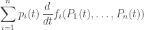
Abstract. Suppose we have n different types of self-replicating entity, with the population of the ith type changing at a rate equal to times the fitness of that type. Suppose the fitness is any continuous function of all the populations . Let be the fraction of replicators that are of the ith type. Then is a time-dependent probability distribution, and we prove that its speed as measured by the Fisher information metric equals the variance in fitness. In rough terms, this says that the speed at which information is updated through natural selection equals the variance in fitness. This result can be seen as a modified version of Fisher’s fundamental theorem of natural selection. We compare it to Fisher’s original result as interpreted by Price, Ewens and Edwards.

Introduction

In 1930, Fisher stated his “fundamental theorem of natural selection” as follows:

The rate of increase in fitness of any organism at any time is equal to its genetic variance in fitness at that time

Some tried to make this statement precise as follows:

The time derivative of the mean fitness of a population equals the variance of its fitness.

But this is only true under very restrictive conditions, so a controversy was ignited.

An interesting resolution was proposed by Price, and later amplified by Ewens and Edwards. We can formalize their idea as follows. Suppose we have n types of self-replicating entity, and idealize the population of the ith type as a real-valued function . Suppose

where the fitness is a differentiable function of the populations of every type of replicator. The mean fitness at time is

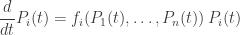
where is the fraction of replicators of the ith type:

By the product rule, the rate of change of the mean fitness is the sum of two terms:

The first of these two terms equals the variance of the fitness at time t. We give the easy proof in Theorem 1. Unfortunately, the conceptual significance of this first term is much less clear than that of the total rate of change of mean fitness. Ewens concluded that “the theorem does not provide the substantial biological statement that Fisher claimed”.

But there is another way out, based on an idea Fisher himself introduced in 1922: Fisher information. Fisher information gives rise to a Riemannian metric on the space of probability distributions on a finite set, called the ‘Fisher information metric’—or in the context of evolutionary game theory, the ‘Shahshahani metric’. Using this metric we can define the speed at which a time-dependent probability distribution changes with time. We call this its ‘Fisher speed’. Under just the assumptions already stated, we prove in Theorem 2 that the Fisher speed of the probability distribution

is the variance of the fitness at time t.

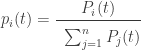
As explained by Harper, natural selection can be thought of as a learning process, and studied using ideas from information geometry—that is, the geometry of the space of probability distributions. As changes with time, the rate at which information is updated is closely connected to its Fisher speed. Thus, our revised version of the fundamental theorem of natural selection can be loosely stated as follows:

As a population changes with time, the rate at which information is updated equals the variance of fitness.

The precise statement, with all the hypotheses, is in Theorem 2. But one lesson is this: variance in fitness may not cause ‘progress’ in the sense of increased mean fitness, but it does cause change!

For more details in a user-friendly blog format, read the whole series:

• Part 1: the obscurity of Fisher’s original paper.

• Part 2: a precise statement of Fisher’s fundamental theorem of natural selection, and conditions under which it holds.

• Part 3: a modified version of the fundamental theorem of natural selection, which holds much more generally.

• Part 4: my paper on the fundamental theorem of natural selection.

Nonequilibrium Thermodynamics in Biology (Part 2)

Larry Li, Bill Cannon and I ran a session on non-equilibrium thermodynamics in biology at SMB2021, the annual meeting of the Society for Mathematical Biology. You can see talk slides here!

Here’s the basic idea:

Since Lotka, physical scientists have argued that living things belong to a class of complex and orderly systems that exist not despite the second law of thermodynamics, but because of it. Life and evolution, through natural selection of dissipative structures, are based on non-equilibrium thermodynamics. The challenge is to develop an understanding of what the respective physical laws can tell us about flows of energy and matter in living systems, and about growth, death and selection. This session addresses current challenges including understanding emergence, regulation and control across scales, and entropy production, from metabolism in microbes to evolving ecosystems.

Click on the links to see slides for most of the talks:

• Persistence, permanence, and global stability in reaction network models: some results inspired by thermodynamic principles
Gheorghe Craciun, University of Wisconsin–Madison

The standard mathematical model for the dynamics of concentrations in biochemical networks is called mass-action kinetics. We describe mass-action kinetics and discuss the connection between special classes of mass-action systems (such as detailed balanced and complex balanced systems) and the Boltzmann equation. We also discuss the connection between the ‘global attractor conjecture’ for complex balanced mass-action systems and Boltzmann’s H-theorem. We also describe some implications for biochemical mechanisms that implement noise filtering and cellular homeostasis.

• The principle of maximum caliber of nonequilibria
Ken Dill, Stony Brook University

Maximum Caliber is a principle for inferring pathways and rate distributions of kinetic processes. The structure and foundations of MaxCal are much like those of Maximum Entropy for static distributions. We have explored how MaxCal may serve as a general variational principle for nonequilibrium statistical physics—giving well-known results, such as the Green-Kubo relations, Onsager’s reciprocal relations and Prigogine’s Minimum Entropy Production principle near equilibrium, but is also applicable far from equilibrium. I will also discuss some applications, such as finding reaction coordinates in molecular simulations non-linear dynamics in gene circuits, power-law-tail distributions in ‘social-physics’ networks, and others.

• Nonequilibrium biomolecular information processes
Pierre Gaspard, Université libre de Bruxelles

Nearly 70 years have passed since the discovery of DNA structure and its role in coding genetic information. Yet, the kinetics and thermodynamics of genetic information processing in DNA replication, transcription, and translation remain poorly understood. These template-directed copolymerization processes are running away from equilibrium, being powered by extracellular energy sources. Recent advances show that their kinetic equations can be exactly solved in terms of so-called iterated function systems. Remarkably, iterated function systems can determine the effects of genome sequence on replication errors, up to a million times faster than kinetic Monte Carlo algorithms. With these new methods, fundamental links can be established between molecular information processing and the second law of thermodynamics, shedding a new light on genetic drift, mutations, and evolution.

• Nonequilibrium dynamics of disturbed ecosystems
John Harte, University of California, Berkeley

The Maximum Entropy Theory of Ecology (METE) predicts the shapes of macroecological metrics in relatively static ecosystems, across spatial scales, taxonomic categories, and habitats, using constraints imposed by static state variables. In disturbed ecosystems, however, with time-varying state variables, its predictions often fail. We extend macroecological theory from static to dynamic, by combining the MaxEnt inference procedure with explicit mechanisms governing disturbance. In the static limit, the resulting theory, DynaMETE, reduces to METE but also predicts a new scaling relationship among static state variables. Under disturbances, expressed as shifts in demographic, ontogenic growth, or migration rates, DynaMETE predicts the time trajectories of the state variables as well as the time-varying shapes of macroecological metrics such as the species abundance distribution and the distribution of metabolic rates over
individuals. An iterative procedure for solving the dynamic theory is presented. Characteristic signatures of the deviation from static predictions of macroecological patterns are shown to result from different kinds of disturbance. By combining MaxEnt inference with explicit dynamical mechanisms of disturbance, DynaMETE is a candidate theory of macroecology for ecosystems responding to anthropogenic or natural disturbances.

• Stochastic chemical reaction networks
Supriya Krishnamurthy, Stockholm University

The study of chemical reaction networks (CRN’s) is a very active field. Earlier well-known results (Feinberg Chem. Enc. Sci. 42 2229 (1987), Anderson et al Bull. Math. Biol. 72 1947 (2010)) identify a topological quantity called deficiency, easy to compute for CRNs of any size, which, when exactly equal to zero, leads to a unique factorized (non-equilibrium) steady-state for these networks. No general results exist however for the steady states of non-zero-deficiency networks. In recent work, we show how to write the full moment-hierarchy for any non-zero-deficiency CRN obeying mass-action kinetics, in terms of equations for the factorial moments. Using these, we can recursively predict values for lower moments from higher moments, reversing the procedure usually used to solve moment hierarchies. We show, for non-trivial examples, that in this manner we can predict any moment of interest, for CRN’s with non-zero deficiency and non-factorizable steady states. It is however an open question how scalable these techniques are for large networks.

• Heat flows adjust local ion concentrations in favor of prebiotic chemistry
Christof Mast, Ludwig-Maximilians-Universität München

Prebiotic reactions often require certain initial concentrations of ions. For example, the activity of RNA enzymes requires a lot of divalent magnesium salt, whereas too much monovalent sodium salt leads to a reduction in enzyme function. However, it is known from leaching experiments that prebiotically relevant geomaterial such as basalt releases mainly a lot of sodium and only little magnesium. A natural solution to this problem is heat fluxes through thin rock fractures, through which magnesium is actively enriched and sodium is depleted by thermogravitational convection and thermophoresis. This process establishes suitable conditions for ribozyme function from a basaltic leach. It can take place in a spatially distributed system of rock cracks and is therefore particularly stable to natural fluctuations and disturbances.

• Deficiency of chemical reaction networks and thermodynamics
Matteo Polettini, University of Luxembourg

Deficiency is a topological property of a Chemical Reaction Network linked to important dynamical features, in particular of deterministic fixed points and of stochastic stationary states. Here we link it to thermodynamics: in particular we discuss the validity of a strong vs. weak zeroth law, the existence of time-reversed mass-action kinetics, and the possibility to formulate marginal fluctuation relations. Finally we illustrate some subtleties of the Python module we created for MCMC stochastic simulation of CRNs, soon to be made public.

• Large deviations theory and emergent landscapes in biological dynamics
Hong Qian, University of Washington

The mathematical theory of large deviations provides a nonequilibrium thermodynamic description of complex biological systems that consist of heterogeneous individuals. In terms of the notions of stochastic elementary reactions and pure kinetic species, the continuous-time, integer-valued Markov process dictates a thermodynamic structure that generalizes (i) Gibbs’ microscopic chemical thermodynamics of equilibrium matters to nonequilibrium small systems such as living cells and tissues; and (ii) Gibbs’ potential function to the landscapes for biological dynamics, such as that of C. H. Waddington and S. Wright.

• Using the maximum entropy production principle to understand and predict microbial biogeochemistry
Joseph Vallino, Marine Biological Laboratory, Woods Hole

Natural microbial communities contain billions of individuals per liter and can exceed a trillion cells per liter in sediments, as well as harbor thousands of species in the same volume. The high species diversity contributes to extensive metabolic functional capabilities to extract chemical energy from the environment, such as methanogenesis, sulfate reduction, anaerobic photosynthesis, chemoautotrophy, and many others, most of which are only expressed by bacteria and archaea. Reductionist modeling of natural communities is problematic, as we lack knowledge on growth kinetics for most organisms and have even less understanding on the mechanisms governing predation, viral lysis, and predator avoidance in these systems. As a result, existing models that describe microbial communities contain dozens to hundreds of parameters, and state variables are extensively aggregated. Overall, the models are little more than non-linear parameter fitting exercises that have limited, to no, extrapolation potential, as there are few principles governing organization and function of complex self-assembling systems. Over the last decade, we have been developing a systems approach that models microbial communities as a distributed metabolic network that focuses on metabolic function rather than describing individuals or species. We use an optimization approach to determine which metabolic functions in the network should be up regulated versus those that should be down regulated based on the non-equilibrium thermodynamics principle of maximum entropy production (MEP). Derived from statistical mechanics, MEP proposes that steady state systems will likely organize to maximize free energy dissipation rate. We have extended this conjecture to apply to non-steady state systems and have proposed that living systems maximize entropy production integrated over time and space, while non-living systems maximize instantaneous entropy production. Our presentation will provide a brief overview of the theory and approach, as well as present several examples of applying MEP to describe the biogeochemistry of microbial systems in laboratory experiments and natural ecosystems.

• Reduction and the quasi-steady state approximation
Carsten Wiuf, University of Copenhagen

Chemical reactions often occur at different time-scales. In applications of chemical reaction network theory it is often desirable to reduce a reaction network to a smaller reaction network by elimination of fast species or fast reactions. There exist various techniques for doing so, e.g. the Quasi-Steady-State Approximation or the Rapid Equilibrium Approximation. However, these methods are not always mathematically justifiable. Here, a method is presented for which (so-called) non-interacting species are eliminated by means of QSSA. It is argued that this method is mathematically sound. Various examples are given (Michaelis-Menten mechanism, two-substrate mechanism, …) and older related techniques from the 50s and 60s are briefly discussed.