I’d like to continue talking about this paper:
• John Baez and Jade Master, Open Petri nets, Mathematical Structures in Computer Science, 30 (2020), 314–341.
Last time I explained, in a sketchy way, the double category of open Petri nets. This time I’d like to describe a ‘semantics’ for open Petri nets.
In his famous thesis Functorial Semantics of Algebraic Theories, Lawvere introduced the idea that semantics, as a map from expressions to their meanings, should be a functor between categories. This has been generalized in many directions, and the same idea works for double categories. So, we describe our semantics for open Petri nets as a map

from our double category of open Petri nets to a double category of relations. This map sends any open Petri net to its ‘reachability relation’.
In Petri net theory, a marking of a set 

For example, here’s a Petri net from chemistry:

Here’s a marking of its places:

But using the transitions, we can repeatedly change the marking. We started with one atom of carbon, one molecule of oxygen, one molecule of sodium hydroxide and one molecule of hydrochloric acid. But they can turn into one molecule of carbon dioxide, one molecule of sodium hydroxide and one molecule of hydrochloric acid:

These can then turn into one molecule of sodium bicarbonate and one molecule of hydrochloric acid:

Then these can turn into one molecule of carbon dioxide, one molecule of water and one molecule of sodium chloride:

People say one marking is reachable from another if you can get it using a finite sequence of transitions in this manner. (Our paper explains this well-known notion more formally.) In this example every marking has 0 or 1 tokens in each place. But that’s not typical: in general we could have any natural number of tokens in each place, so long as the total number of tokens is finite.
Our paper adapts the concept of reachability to open Petri nets. Let ![\mathbb{N}[X]](https://s0.wp.com/latex.php?latex=%5Cmathbb%7BN%7D%5BX%5D&bg=ffffff&fg=333333&s=0&c=20201002)

![\blacksquare P \subseteq \mathbb{N}[X] \times \mathbb{N}[Y]](https://s0.wp.com/latex.php?latex=%5Cblacksquare+P+%5Csubseteq+%5Cmathbb%7BN%7D%5BX%5D+%5Ctimes+%5Cmathbb%7BN%7D%5BY%5D+&bg=ffffff&fg=333333&s=0&c=20201002)
This relation holds when we can take a given marking of 


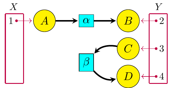
For example, consider this open Petri net


Here is a marking of

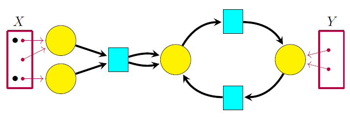
We can feed these tokens into 

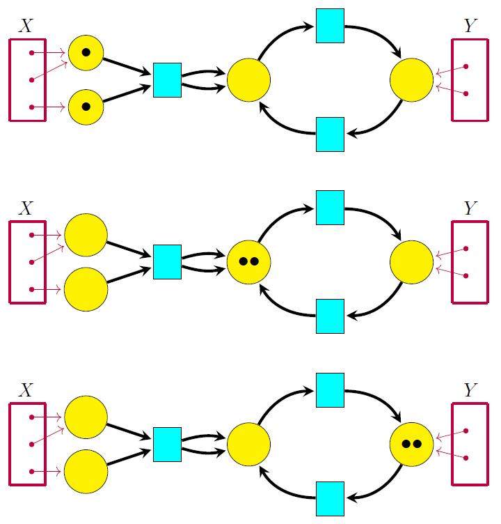
They can then pop out into
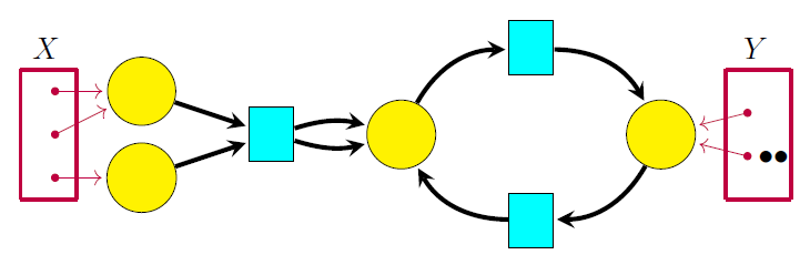
This gives a marking of 
The main result of our paper is that the map sending an open Petri net 
where 

I can give you a bit more detail on those double categories, and also give you a clue about what ‘lax’ means, without it becoming too stressful.
Last time I said the double category
• sets 
• functions 
• open Petri nets
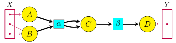
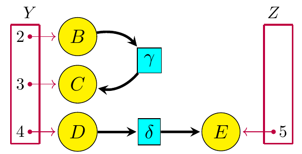
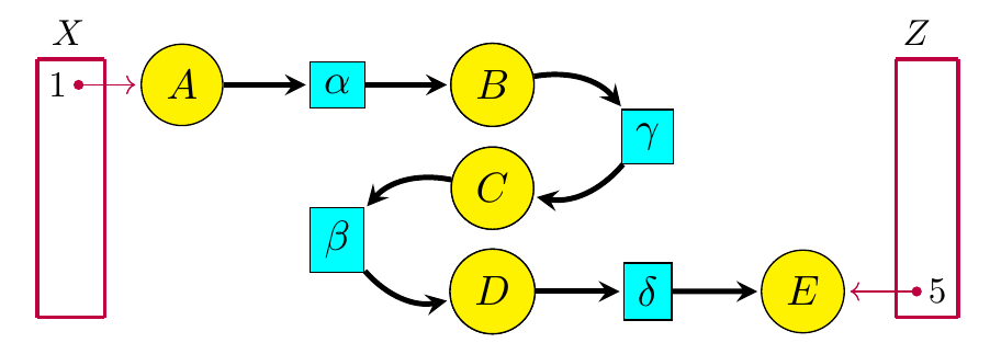
• morphisms between open Petri nets as 2-morphisms—an example would be the visually obvious map from this open Petri net:
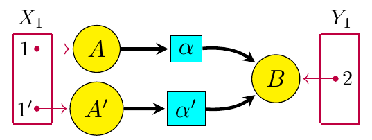
to this one:
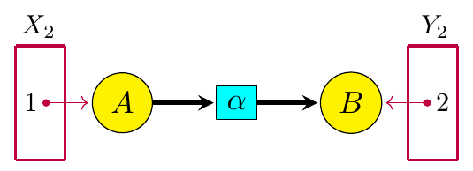
What about 
• sets
• functions
• relations 
• maps between relations as 2-morphisms. Here a map between relations is a square
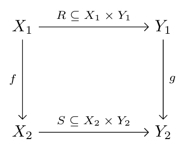
that obeys

So, the idea of the reachability semantics is that it maps:
• any set
• any function
![\mathbb{N}(f) \colon \mathbb{N}[X] \to \mathbb{N}[Y]](https://s0.wp.com/latex.php?latex=%5Cmathbb%7BN%7D%28f%29+%5Ccolon+%5Cmathbb%7BN%7D%5BX%5D+%5Cto+%5Cmathbb%7BN%7D%5BY%5D&bg=ffffff&fg=333333&s=0&c=20201002)
(Yes, 
• any open Petri net
![\blacksquare P \colon \mathbb{N}[X] \to \mathbb{N}[Y]](https://s0.wp.com/latex.php?latex=%5Cblacksquare+P+%5Ccolon+%5Cmathbb%7BN%7D%5BX%5D+%5Cto+%5Cmathbb%7BN%7D%5BY%5D&bg=ffffff&fg=333333&s=0&c=20201002)
• any morphism between Petri nets to the obvious map between their reachability relations.
Especially if you draw some examples, all this seems quite reasonable and nice. But it’s important to note that 


Instead, we just have

It’s easy to see why. Take
and take 
Then their composite 
It’s easy to see that 


In our paper, Jade and I conjecture that we get
if we restrict the reachability semantics to a certain specific sub-double category of
Finally, besides showing that
is a lax double functor, we also show that it’s symmetric monoidal. This means that the reachability semantics works as you’d expect when you run two open Petri nets ‘in parallel’.
In a way, the most important thing about our paper is that it illustrates some methods to study semantics for symmetric monoidal double categories. Kenny Courser and I will describe these methods more generally in our paper “Structured cospans.” They can be applied to timed Petri nets, colored Petri nets, and various other kinds of Petri nets. One can also develop a reachability semantics for open Petri nets that are glued together along transitions as well as places.
I hear that the company Statebox wants these and other generalizations. We aim to please—so we’d like to give it a try.
Next time I’ll wrap up this little series of posts by explaining how Petri nets give symmetric monoidal categories.
• Part 1: the double category of open Petri nets.
• Part 2: the reachability semantics for open Petri nets.
• Part 3: the free symmetric monoidal category on a Petri net.


How would you analyze a “self” loop, where an arrow from a transition goes to a place (self) thence back to the originating transition– with other arrows possible? (I had to do that once when simulating a factory system using diagrams of Petri nets automatically coded into Smalltalk80. Without the self loop, multiple parts entering the queue for a machine would spawn multiple instances of the transition in multiple threads, while in the factory the machine would only process one part at a time.)
A loop like this describes a transition where something turns into itself. Such transitions can be removed from a Petri net without affecting reachability.
If reachability is our only concern, then certainly we can ignore self loops. But if thermodynamics is of any concern, self loops are a way to model a thermodynamic engine. In a factory, the engine doesn’t start when you put a part in the input queuing place to a transition that models a machine. The thermodynamic engine starts when you put a token in the “self” place. To stop the thermodynamic engine, remove the token from the “self” place. Regarding chemistry, that might be of interest for models of biological systems, which involve thermodynamics.
Unless I misunderstand reachability (which is quite possible), then the laxness should be , rather than the other way around. That is, if something's reachable by going through
  after going through
  , then it's reachable by going through
  , but additional zigzag reachings may also exist in
  .
.
Also, shouldn't the chemistry diagrams have some nodes with more than mark in them? Not in the original diagram, but in the later ones, if each is supposed to be reachable from the previous one.
I should have written I’ll fix that—thanks! I hope I didn’t get it twisted around in the actual paper.
I don’t think so. We start with one atom of carbon, one molecule of oxygen, one molecule of sodium hydroxide and one molecule of hydrochloric acid:
They turn into one molecule of carbon dioxide, one molecule of sodium hydroxide and one molecule of hydrochloric acid:
These turn into one molecule of sodium bicarbonate and one molecule of hydrochloric acid:
These turn into one molecule of carbon dioxide, one molecule of water and one molecule of sodium chloride:
So, there’s always at most one token in each place in this story. That’s not true for all such stories, so this example is unrepresentative, but I think I’ve got the chemistry basically right: atoms of each kind are being conserved.
Thanks, l understand what the chemical example is showing now.
Okay, good. I’ve added my explanation to the blog post to make it clearer.
(I’m saying this so nobody wonders why you needed to have it explained twice. )
)
I wonder if this is relevant to reasoning about dropping grains of sand on an Abelian sandpile. Ie could it show that all points on lattice are reachable from dropping grains on a single tile repeatedly, or more interestingly, would it be able to tell you things about interference patterns caused by dropping grains at two points separated by n cells simultaneously, etc. Would it cause an problem in applying these techniques if the lattice is infinite instead of a finite number of cells?
This talk on structured cospans and Petri nets is the second of a two-part series, but it should be understandable on its own. The first part is on structured cospans and double categories.
You can see my talk live on YouTube here, with simultaneous discussion on the Category Theory Community Server. (To join this, click here.) The talk will be recorded and remain available on YouTube.
You can already see the slides here.