Struggles with the Continuum (Part 3)

In these posts, we’re seeing how our favorite theories of physics deal with the idea that space and time are a continuum, with points described as lists of real numbers. We’re not asking if this idea is true: there’s no clinching evidence to answer that question, so it’s too easy to let ones philosophical prejudices choose the answer. Instead, we’re looking to see what problems this idea causes, and how physicists have struggled to solve them.

We started with the Newtonian mechanics of point particles attracting each other with an inverse square force law. We found strange ‘runaway solutions’ where particles shoot to infinity in a finite amount of time by converting an infinite amount of potential energy into kinetic energy.

Then we added quantum mechanics, and we saw this problem went away, thanks to the uncertainty principle.

Now let’s take away quantum mechanics and add special relativity. Now our particles can’t go faster than light. Does this help?

Point particles interacting with the electromagnetic field

Special relativity prohibits instantaneous action at a distance. Thus, most physicists believe that special relativity requires that forces be carried by fields, with disturbances in these fields propagating no faster than the speed of light. The argument for this is not watertight, but we seem to actually see charged particles transmitting forces via a field, the electromagnetic field—that is, light. So, most work on relativistic interactions brings in fields.

Classically, charged point particles interacting with the electromagnetic field are described by two sets of equations: Maxwell’s equations and the Lorentz force law. The first are a set of differential equations involving:

• the electric field and mangetic field which in special relativity are bundled together into the electromagnetic field and

• the electric charge density and current density which are bundled into another field called the ‘four-current’

By themselves, these equations are not enough to completely determine the future given initial conditions. In fact, you can choose and freely, subject to the conservation law

For any such choice, there exists a solution of Maxwell’s equations for given initial values for and that obey these equations at

Thus, to determine the future given initial conditions, we also need equations that say what and will do. For a collection of charged point particles, they are determined by the curves in spacetime traced out by these particles. The Lorentz force law says that the force on a particle of charge is

where is the particle’s velocity and and are evaluated at the particle’s location. From this law we can compute the particle’s acceleration if we know its mass.

The trouble starts when we try to combine Maxwell’s equations and the Lorentz force law in a consistent way, with the goal being to predict the future behavior of the and fields, together with particles’ positions and velocities, given all these quantities at Attempts to do this began in the late 1800s. The drama continues today, with no definitive resolution! You can find good accounts, available free online, by Feynman and by Janssen and Mecklenburg. Here we can only skim the surface.

The first sign of a difficulty is this: the charge density and current associated to a charged particle are singular, vanishing off the curve it traces out in spacetime but ‘infinite’ on this curve. For example, a charged particle at rest at the origin has

where is the Dirac delta and is the particle’s charge. This in turn forces the electric field to be singular at the origin. The simplest solution of Maxwell’s equations consisent with this choice of and is

where is a unit vector pointing away from the origin and is a constant called the permittivity of free space.

In short, the electric field is ‘infinite’, or undefined, at the particle’s location. So, it is unclear how to define the ‘self-force’ exerted by the particle’s own electric field on itself. The formula for the electric field produced by a static point charge is really just our old friend, the inverse square law. Since we had previously ignored the force of a particle on itself, we might try to continue this tactic now. However, other problems intrude.

In relativistic electrodynamics, the electric field has energy density equal to

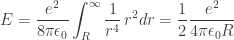
Thus, the total energy of the electric field of a point charge at rest is proportional to

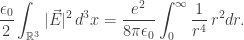
But this integral diverges near so the electric field of a charged particle has an infinite energy!

How, if at all, does this cause trouble when we try to unify Maxwell’s equations and the Lorentz force law? It helps to step back in history. In 1902, the physicist Max Abraham assumed that instead of a point, an electron is a sphere of radius with charge evenly distributed on its surface. Then the energy of its electric field becomes finite, namely:

where is the electron’s charge.

Abraham also computed the extra momentum a moving electron of this sort acquires due to its electromagnetic field. He got it wrong because he didn’t understand Lorentz transformations. In 1904 Lorentz did the calculation right. Using the relationship between velocity, momentum and mass, we can derive from his result a formula for the ‘electromagnetic mass’ of the electron:

where is the speed of light. We can think of this as the extra mass an electron acquires by carrying an electromagnetic field along with it.

Putting the last two equations together, these physicists obtained a remarkable result:

Then, in 1905, a fellow named Einstein came along and made it clear that the only reasonable relation between energy and mass is

What had gone wrong?

In 1906, Poincaré figured out the problem. It is not a computational mistake, nor a failure to properly take special relativity into account. The problem is that like charges repel, so if the electron were a sphere of charge it would explode without something to hold it together. And that something—whatever it is—might have energy. But their calculation ignored that extra energy.

In short, the picture of the electron as a tiny sphere of charge, with nothing holding it together, is incomplete. And the calculation showing together with special relativity saying shows that this incomplete picture is inconsistent. At the time, some physicists hoped that all the mass of the electron could be accounted for by the electromagnetic field. Their hopes were killed by this discrepancy.

Nonetheless it is interesting to take the energy computed above, set it equal to where is the electron’s observed mass, and solve for the radius The answer is

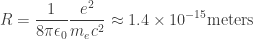
In the early 1900s, this would have been a remarkably tiny distance: times the Bohr radius of a hydrogen atom. By now we know this is roughly the radius of a proton. We know that electrons are not spheres of this size. So at present it makes more sense to treat the calculations so far as a prelude to some kind of limiting process where we take These calculations teach us two lessons.

First, the electromagnetic field energy approaches as we let so we will be hard pressed to take this limit and get a well-behaved physical theory. One approach is to give a charged particle its own ‘bare mass’ in addition to the mass arising from electromagnetic field energy, in a way that depends on Then as we take the limit we can let in such a way that approaches a chosen limit the physical mass of the point particle. This is an example of ‘renormalization’.

Second, it is wise to include conservation of energy-momentum as a requirement in addition to Maxwell’s equations and the Lorentz force law. Here is a more sophisticated way to phrase Poincaré’s realization. From the electromagnetic field one can compute a ‘stress-energy tensor’ which describes the flow of energy and momentum through spacetime. If all the energy and momentum of an object comes from its electromagnetic field, you can compute them by integrating over the hypersurface You can prove that the resulting 4-vector transforms correctly under Lorentz transformations if you assume the stress-energy tensor has vanishing divergence: This equation says that energy and momentum are locally conserved. However, this equation fails to hold for a spherical shell of charge with no extra forces holding it together. In the absence of extra forces, it violates conservation of momentum for a charge to feel an electromagnetic force yet not accelerate.

So far we have only discussed the simplest situation: a single charged particle at rest, or moving at a constant velocity. To go further, we can try to compute the acceleration of a small charged sphere in an arbitrary electromagnetic field. Then, by taking the limit as the radius of the sphere goes to zero, perhaps we can obtain the law of motion for a charged point particle.

In fact this whole program is fraught with difficulties, but physicists boldly go where mathematicians fear to tread, and in a rough way this program was carried out already by Abraham in 1905. His treatment of special relativistic effects was wrong, but these were easily corrected; the real difficulties lie elsewhere. In 1938 his calculations were carried out much more carefully—though still not rigorously—by Dirac. The resulting law of motion is thus called the ‘Abraham–Lorentz–Dirac force law’.

There are three key ways in which this law differs from our earlier naive statement of the Lorentz force law:

• We must decompose the electromagnetic field in two parts, the ‘external’ electromagnetic field and the field produced by the particle:

Here is a solution Maxwell equations with while is computed by convolving the particle’s 4-current with a function called the ‘retarded Green’s function’. This breaks the time-reversal symmetry of the formalism so far, ensuring that radiation emitted by the particle moves outward as increases. We then decree that the particle only feels a Lorentz force due to not This avoids the problem that becomes infinite along the particle’s path as

• Maxwell’s equations say that an accelerating charged particle emits radiation, which carries energy-momentum. Conservation of energy-momentum implies that there is a compensating force on the charged particle. This is called the ‘radiation reaction’. So, in addition to the Lorentz force, there is a radiation reaction force.

• As we take the limit we must adjust the particle’s bare mass in such a way that its physical mass is held constant. This involves letting as

It is easiest to describe the Abraham–Lorentz–Dirac force law using standard relativistic notation. So, we switch to units where and equal 1, let denote the spacetime coordinates of a point particle, and use a dot to denote the derivative with respect to proper time. Then the Abraham–Lorentz–Dirac force law says

The first term at right is the Lorentz force, which looks more elegant in this new notation. The second term is fairly intuitive: it acts to reduce the particle’s velocity at a rate proportional to its velocity (as one would expect from friction), but also proportional to the squared magnitude of its acceleration. This is the ‘radiation reaction’.

The last term, called the ‘Schott term’, is the most shocking. Unlike all familiar laws in classical mechanics, it involves the third derivative of the particle’s position!

This seems to shatter our original hope of predicting the electromagnetic field and the particle’s position and velocity given their initial values. Now it seems we need to specify the particle’s initial position, velocity and acceleration.

Furthermore, unlike Maxwell’s equations and the original Lorentz force law, the Abraham–Lorentz–Dirac force law is not symmetric under time reversal. If we take a solution and replace with the result is not a solution. Like the force of friction, radiation reaction acts to make a particle lose energy as it moves into the future, not the past.

The reason is that our assumptions have explicitly broken time symmetry. The splitting says that a charged accelerating particle radiates into the future, creating the field and is affected only by the remaining electromagnetic field

Worse, the Abraham–Lorentz–Dirac force law has counterintuitive solutions. Suppose for example that Besides the expected solutions where the particle’s velocity is constant, there are solutions for which the particle accelerates indefinitely, approaching the speed of light! These are called ‘runaway solutions’. In these runaway solutions, the acceleration as measured in the frame of reference of the particle grows exponentially with the passage of proper time.

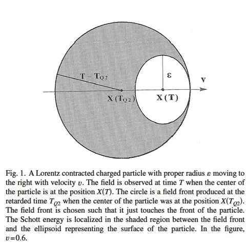
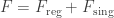
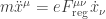
So, the notion that special relativity might help us avoid the pathologies of Newtonian point particles interacting gravitationally—five-body solutions where particles shoot to infinity in finite time—is cruelly mocked by the Abraham–Lorentz–Dirac force law. Particles cannot move faster than light, but even a single particle can extract an arbitrary amount of energy-momentum from the electromagnetic field in its immediate vicinity and use this to propel itself forward at speeds approaching that of light. The energy stored in the field near the particle is sometimes called ‘Schott energy’.

Thanks to the Schott term in the Abraham–Lorentz–Dirac force law, the Schott energy can be converted into kinetic energy for the particle. The details of how this work are nicely discussed in a paper by Øyvind Grøn, so click the link and read that if you’re interested. I’ll just show you a picture from that paper:

So even one particle can do crazy things! But worse, suppose we generalize the framework to include more than one particle. The arguments for the Abraham–Lorentz–Dirac force law can be generalized to this case. The result is simply that each particle obeys this law with an external field that includes the fields produced by all the other particles. But a problem appears when we use this law to compute the motion of two particles of opposite charge. To simplify the calculation, suppose they are located symmetrically with respect to the origin, with equal and opposite velocities and accelerations. Suppose the external field felt by each particle is solely the field created by the other particle. Since the particles have opposite charges, they should attract each other. However, one can prove they will never collide. In fact, if at any time they are moving towards each other, they will later turn around and move away from each other at ever-increasing speed!

This fact was discovered by C. Jayaratnam Eliezer in 1943. It is so counterintuitive that several proofs were required before physicists believed it.

None of these strange phenomena have ever been seen experimentally. Faced with this problem, physicists have naturally looked for ways out. First, why not simply cross out the term in the Abraham–Lorentz–Dirac force? Unfortunately the resulting simplified equation

has only trivial solutions. The reason is that with the particle’s path parametrized by proper time, the vector has constant length, so the vector is orthogonal to . So is the vector because is an antisymmetric tensor. So, the last term must be zero, which implies which in turn implies that all three terms must vanish.

Another possibility is that some assumption made in deriving the Abraham–Lorentz–Dirac force law is incorrect. Of course the theory is physically incorrect, in that it ignores quantum mechanics and other things, but that is not the issue. The issue here is one of mathematical physics, of trying to formulate a well-behaved classical theory that describes charged point particles interacting with the electromagnetic field. If we can prove this is impossible, we will have learned something. But perhaps there is a loophole. The original arguments for the Abraham–Lorentz–Dirac force law are by no means mathematically rigorous. They involve a delicate limiting procedure, and approximations that were believed, but not proved, to become perfectly accurate in the limit. Could these arguments conceal a mistake?

Calculations involving a spherical shell of charge has been improved by a series of authors, and nicely summarized by Fritz Rohrlich. In all these calculations, nonlinear powers of the acceleration and its time derivatives are neglected, and one hopes this is acceptable in the limit.

Dirac, struggling with renormalization in quantum field theory, took a different tack. Instead of considering a sphere of charge, he treated the electron as a point from the very start. However, he studied the flow of energy-momentum across the surface of a tube of radius centered on the electron’s path. By computing this flow in the limit and using conservation of energy-momentum, he attempted to derive the force on the electron. He did not obtain a unique result, but the simplest choice gives the Abraham–Lorentz–Dirac equation. More complicated choices typically involve nonlinear powers of the acceleration and its time derivatives.

Since this work, many authors have tried to simplify Dirac’s rather complicated calculations and clarify his assumptions. This book is a good guide:

• Stephen Parrott, Relativistic Electrodynamics and Differential Geometry, Springer, Berlin, 1987.

But more recently, Jerzy Kijowski and some coauthors have made impressive progress in a series of papers that solve many of the problems we have described.

Kijowski’s key idea is to impose conditions on precisely how the electromagnetic field is allowed to behave near the path traced out by a charged point particle. He breaks the field into a ‘regular’ part and a ‘singular’ part:

Here is smooth everywhere, while is singular near the particle’s path, but only in a carefully prescribed way. Roughly, at each moment, in the particle’s instantaneous rest frame, the singular part of its electric field consists of the familiar part proportional to together with a part proportional to which depends on the particle’s acceleration. No other singularities are allowed!

On the one hand, this eliminates the ambiguities mentioned earlier: in the end, there are no ‘nonlinear powers of the acceleration and its time derivatives’ in Kijowski’s force law. On the other hand, this avoids breaking time reversal symmetry, as the earlier splitting did.

Next, Kijowski defines the energy-momentum of a point particle to be where is its physical mass. He defines the energy-momentum of the electromagnetic field to be just that due to not This amounts to eliminating the infinite ‘electromagnetic mass’ of the charged particle. He then shows that Maxwell’s equations and conservation of total energy-momentum imply an equation of motion for the particle!

This equation is very simple:

It is just the Lorentz force law! Since the troubling Schott term is gone, this is a second-order differential equation. So we can hope that to predict the future behavior of the electromagnetic field, together with the particle’s position and velocity, given all these quantities at

And indeed this is true! In 1998, together with Gittel and Zeidler, Kijowski proved that initial data of this sort, obeying the careful restrictions on allowed singularities of the electromagnetic field, determine a unique solution of Maxwell’s equations and the Lorentz force law, at least for a short amount of time. Even better, all this remains true for any number of particles.

There are some obvious questions to ask about this new approach. In the Abraham–Lorentz–Dirac force law, the acceleration was an independent variable that needed to be specified at along with position and momentum. This problem disappears in Kijowski’s approach. But how?

We mentioned that the singular part of the electromagnetic field, depends on the particle’s acceleration. But more is true: the particle’s acceleration is completely determined by So, the particle’s acceleration is not an independent variable because it is encoded into the electromagnetic field.

Another question is: where did the radiation reaction go? The answer is: we can see it if we go back and decompose the electromagnetic field as as we had before. If we take the law

and rewrite it in terms of we recover the original Abraham–Lorentz–Dirac law, including the radiation reaction term and Schott term.

Unfortunately, this means that ‘pathological’ solutions where particles extract arbitrary amounts of energy from the electromagnetic field are still possible. A related problem is that apparently nobody has yet proved solutions exist for all time. Perhaps a singularity worse than the allowed kind could develop in a finite amount of time—for example, when particles collide.

So, classical point particles interacting with the electromagnetic field still present serious challenges to the physicist and mathematician. When you have an infinitely small charged particle right next to its own infinitely strong electromagnetic field, trouble can break out very easily!

Particles without fields

Finally, I should also mention attempts, working within the framework of special relativity, to get rid of fields and have particles interact with each other directly. For example, in 1903 Schwarzschild introduced a framework in which charged particles exert an electromagnetic force on each other, with no mention of fields. In this setup, forces are transmitted not instantaneously but at the speed of light: the force on one particle at one spacetime point depends on the motion of some other particle at spacetime point only if the vector is lightlike. Later Fokker and Tetrode derived this force law from a principle of least action. In 1949, Feynman and Wheeler checked that this formalism gives results compatible with the usual approach to electromagnetism using fields, except for several points:

• Each particle exerts forces only on other particles, so we avoid the thorny issue of how a point particle responds to the electromagnetic field produced by itself.

• There are no electromagnetic fields not produced by particles: for example, the theory does not describe the motion of a charged particle in an ‘external electromagnetic field’.

• The principle of least action guarantees that ‘if affects then affects ’ . So, if a particle at exerts a force on a particle at a point in its future lightcone, the particle at exerts a force on the particle at in its past lightcone. This raises the issue of ‘reverse causality’, which Feynman and Wheeler address.

Besides the reverse causality issue, perhaps one reason this approach has not been more pursued is that it does not admit a Hamiltonian formulation in terms of particle positions and momenta. Indeed, there are a number of ‘no-go theorems’ for relativistic multiparticle Hamiltonians, saying that these can only describe noninteracting particles. So, most work that takes both quantum mechanics and special relativity into account uses fields.

Indeed, in quantum electrodynamics, even the charged point particles are replaced by fields—namely quantum fields! Next time we’ll see whether that helps.

---

• Part 1: introduction; the classical mechanics of gravitating point particles.

• Part 2: the quantum mechanics of point particles.

• Part 3: classical point particles interacting with the electromagnetic field.

• Part 4: quantum electrodynamics.

• Part 5: renormalization in quantum electrodynamics.

• Part 6: summing the power series in quantum electrodynamics.

• Part 7: singularities in general relativity.

• Part 8: cosmic censorship in general relativity; conclusions.