Last time we saw that that nobody yet knows if Newtonian gravity, applied to point particles, truly succeeds in predicting the future. To be precise: for four or more particles, nobody has proved that almost all initial conditions give a well-defined solution for all times!
The problem is related to the continuum nature of space: as particles get arbitrarily close to other, an infinite amount of potential energy can be converted to kinetic energy in a finite amount of time.
I left off by asking if this problem is solve by more sophisticated theories. For example, does the ‘speed limit’ imposed by special relativity help the situation? Or might quantum mechanics help, since it describes particles as ‘probability clouds’, and puts limits on how accurately we can simultaneously know both their position and momentum?
We begin with quantum mechanics, which indeed does help.
The quantum mechanics of charged particles
Few people spend much time thinking about ‘quantum celestial mechanics’—that is, quantum particles obeying Schrödinger’s equation, that attract each other gravitationally, obeying an inverse-square force law. But Newtonian gravity is a lot like the electrostatic force between charged particles. The main difference is a minus sign, which makes like masses attract, while like charges repel. In chemistry, people spend a lot of time thinking about charged particles obeying Schrödinger’s equation, attracting or repelling each other electrostatically. This approximation neglects magnetic fields, spin, and indeed anything related to the finiteness of the speed of light, but it’s good enough explain quite a bit about atoms and molecules.
In this approximation, a collection of charged particles is described by a wavefunction 


where 

Does this equation succeeding in predicting
At any time, we want

where 

In 1951, based on earlier work of Rellich, Kato proved that
The reason, simply put, is the uncertainty principle.
In the classical case, bad things happen because the energy is not bounded below. A pair of classical particles attracting each other with an inverse square force law can have arbitrarily large negative energy, simply by being very close to each other. Since energy is conserved, if you have a way to make some particles get an arbitrarily large negative energy, you can balance the books by letting others get an arbitrarily large positive energy and shoot to infinity in a finite amount of time!
When we switch to quantum mechanics, the energy of any collection of particles becomes bounded below. The reason is that to make the potential energy of two particles large and negative, they must be very close. Thus, their difference in position must be very small. In particular, this difference must be accurately known! Thus, by the uncertainty principle, their difference in momentum must be very poorly known: at least one of its components must have a large standard deviation. This in turn means that the expected value of the kinetic energy must be large.
This must all be made quantitative, to prove that as particles get close, the uncertainty principle provides enough positive kinetic energy to counterbalance the negative potential energy. The Kato–Lax–Milgram–Nelson theorem, a refinement of the original Kato–Rellich theorem, is the key to understanding this issue. The Hamiltonian

where 


Remember that 

By taking 
states

But the fact that the inequality holds even for smaller values of 
To understand what a great triumph this is, one needs to see what could have gone wrong! Suppose space had an extra dimension. In 3-dimensional space, Newtonian gravity obeys an inverse square force law because the area of a sphere is proportional to its radius squared. In 4-dimensional space, the force obeys an inverse cube law:

Using a cube instead of a square here makes the force stronger at short distances, with dramatic effects. For example, even for the classical 2-body problem, the equations of motion no longer ‘almost always’ have a well-defined solution for all times. For an open set of initial conditions, the particles spiral into each other in a finite amount of time!
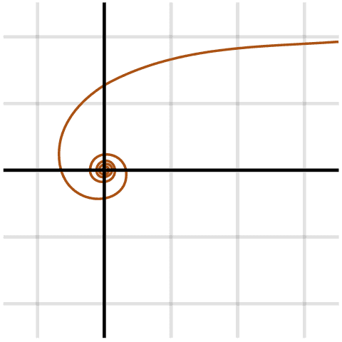 Hyperbolic spiral – a fairly common orbit in an inverse cube force.
The quantum version of this theory is also problematic. The uncertainty principle is not enough to save the day. The inequalities above no longer hold: kinetic energy does not triumph over potential energy. The Hamiltonian is no longer essentially self-adjoint on the set of wavefunctions that I described.
In fact, this Hamiltonian has infinitely many self-adjoint extensions! Each one describes different physics: namely, a different choice of what happens when particles collide. Moreover, when 
The same problems afflict quantum particles interacting by the electrostatic force in 4d space, as long as some of the particles have opposite charges. So, chemistry would be quite problematic in a world with four dimensions of space.
With more dimensions of space, the situation becomes even worse. In fact, this is part of a general pattern in mathematical physics: our struggles with the continuum tend to become worse in higher dimensions. String theory and M-theory may provide exceptions.
Next time we’ll look at what happens to point particles interacting electromagnetically when we take special relativity into account. After that, we’ll try to put special relativity and quantum mechanics together!
For more
For more on the inverse cube force law, see:
• John Baez, The inverse cube force law, Azimuth, 30 August 2015.
It turns out Newton made some fascinating discoveries about this law in his Principia; it has remarkable properties both classically and in quantum mechanics.
The hyperbolic spiral is one of 3 kinds of orbits possible in an inverse cube force; for the others see:
• Cotes’s spiral, Wikipedia.
The picture of a hyperbolic spiral was drawn by Anarkman and Pbroks13 and placed on Wikicommons under a Creative Commons Attribution-Share Alike 3.0 Unported license.
• Part 1: introduction; the classical mechanics of gravitating point particles.
• Part 2: the quantum mechanics of point particles.
• Part 3: classical point particles interacting with the electromagnetic field.
• Part 4: quantum electrodynamics.
• Part 5: renormalization in quantum electrodynamics.
• Part 6: summing the power series in quantum electrodynamics.
• Part 7: singularities in general relativity.
• Part 8: cosmic censorship in general relativity; conclusions.


Wouldn’t it be more accurate to replace the word “known” with “defined”?
You can take either an ontic (“is”) or epistemic (“is known”) stance to the wavefunction. As a quantum subjective Bayesian, I tend to think of the state of a quantum system as serving the same basic role as a probability distribution in probability theory, namely as a summary of our beliefs about what’s going on. But I don’t think there’s a way things “really are”, standing over and above what we know.
Needless to say, these issues don’t matter for what I’m talking about here. So, I should try to use whatever language is the least likely to get people interested in the issue you just raised!
Thus, accuracy is less important to me here than blandness. It’s possible that “defined” will be better in this respect, since it doesn’t bring up any issues of “subjectivity”. Thanks. I’m going to publish this series of blog articles as a paper, but there’s still time to make changes.
(At least to me, “known” makes me imagine that there is one portion of the system which knows something about another portion — not what you meant! But I doubt I’m very representative.)
(To be clear, I always realized you couldn’t possibly have meant “known by a subsystem”; I was just quibbling about how best to describe the uncertainty principle, and about that I do think “know” suggests incorrectly that there is “a way things really are” which is not subject to the same tradeoff in precision. So for me, defined is “blander”, but I have no idea whether that’s true for most readers.)
Bruce Smith writes, citing John Baez:” “In particular, this difference must be accurately known! Thus, by the uncertainty principle, their difference in momentum must be very poorly known …. ”
Wouldn’t it be more accurate to replace the word “known” with “defined”?”
Both are well defined, but the information about their simultaneous position and momentum is only approximate, within the limits set by the Uncertainty Principle. “Known” here refers to experimental observation of the particle or system, “defined” describes the modelling of that system using theoretical descriptions. At least that’s how I’ve understood it. And “known” is limited by the accuracy of the observation – instrumentation and the like, whereas “defined” seems far more concrete.
John, I am mostly paying attention to the prose here. I’m puzzled by “In the classical case, bad things happen because the energy is not bounded below”, juxtaposed with “When we switch to quantum mechanics, the energy of any collection of particles becomes bounded below.”
The first of those sentences concerns only the potential energy part, right? Which suggests that the second sentence does, too. But based on the rest of your discussion, I don’t see anything implying that in the quantum case, the (expected value of) potential energy is in fact bounded below.
Rather, it seems that in both the classical and quantum cases, the PE is not bounded below, but it is balanced by the KE (which arises from motion in the classical case and from momentum uncertainty in the quantum case). Which would seem to imply that in the quantum case, as in the classical case, the (expected value of) KE could get arbitrarily large.
Where did I go off the tracks?
arch1 wrote:
No.
In the classical theory of particles interacting by an attractive 1/r potential, the total energy—potential plus kinetic—is not bounded below. In the quantum theory it is, thanks to the uncertainty principle.
This makes a big difference! This is how the quantum theory avoids the horrible problems that afflict the classical theory.
Aha. Thanks much John, this helps a lot.
Great. If you reread a bit with this in mind, it’ll make more sense.
Classically a positive and negative charged particle can be stationary and as close as you like. Their kinetic energy will be zero and their potential energy will be whatever negative number you desire.
Quantum mechanically, they can’t be very close (with a high probability) while still moving very slow (with a high probability).
In this series we’re looking at mathematical problems that arise in physics due to treating spacetime as a continuum—basically, problems with infinities.
In Part 1 we looked at classical point particles interacting gravitationally. We saw they could convert an infinite amount of potential energy into kinetic energy in a finite time! Then we switched to electromagnetism, and went a bit beyond traditional Newtonian mechanics: in Part 2 we threw quantum mechanics into the mix, and in Part 3 we threw in special relativity. Briefly, quantum mechanics made things better, but special relativity made things worse.
Now let’s throw in both!