Let’s start with a puzzle:
Puzzle. You measure the energy and frequency of some laser light trapped in a mirrored box and use quantum mechanics to compute the expected number of photons in the box. Then someone tells you that you used the wrong value of Planck’s constant in your calculation. Somehow you used a value that was twice the correct value! How should you correct your calculation of the expected number of photons?
I’ll give away the answer to the puzzle below, so avert your eyes if you want to think about it more.
This scenario sounds a bit odd—it’s not very likely that your table of fundamental constants would get Planck’s constant wrong this way. But it’s interesting because once upon a time we didn’t know about quantum mechanics and we didn’t know Planck’s constant. We could still give a reasonably good description of some laser light trapped in a mirrored box: there’s a standing wave solution of Maxwell’s equations that does the job. But when we learned about quantum mechanics we learned to describe this situation using photons. The number of photons we need depends on Planck’s constant.
And while we can’t really change Planck’s constant, mathematical physicists often like to treat Planck’s constant as variable. The limit where Planck’s constant goes to zero is called the ‘classical limit’, where our quantum description should somehow reduce to our old classical description.
Here’s the answer to the puzzle: if you halve Planck’s constant you need to double the number of photons. The reason is that the energy of a photon with frequency 


So, the classical limit is also the limit where the expected number of photons goes to infinity! As the ‘packets of energy’ get smaller, we need more of them to get a certain amount of energy.
This has a nice relationship to what I’d been doing with geometric quantization last time.
I explained how we could systematically replace any classical system considering by a ‘cloned’ version of that system: a collection of identical copies constrained to all lie in the same state. The set of allowed states is the same, but the symplectic structure is multiplied by a constant factor: the number of copies. We can see this as follows: if the phase space of our system is an abstract symplectic manifold 

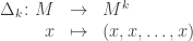
The image is a symplectic submanifold of 


What does this mean for physics?
If we act like physicists instead of mathematicians for a minute and keep track of units, we’ll notice that the naive symplectic structure in classical mechanics has units of action: think 

So: cloning a system, multiplying the number of copies by k, should be related to dividing Planck’s constant by k. And the limit 
Of course this would not convince a mathematician so far, since I’m using a strange mix of ideas from classical mechanics and quantum mechanics! But our approach to geometric quantization makes everything precise. We have a category 


and a functor going back:

which reveals that quantum systems are special classical systems. And last time we saw that there are also ways to ‘clone’ classical and quantum systems.
Our classical systems are more than mere symplectic manifolds: they are projectively normal subvarieties of 

But this cloning process has the same effect on the underlying symplectic manifold: it multiplies the symplectic structure by k.
Similarly, we clone a quantum system by replacing its set of states 


and the ‘obvious squares commute’:


All I’m doing now is giving this math a new physical interpretation: the k-fold cloning process is the same as dividing Planck’s constant by k!
If this seems a bit elusive, we can look at an example like the spin-j particle. In Part 6 we saw that if we clone the state space for the spin-1/2 particle we get the state space for the spin-j particle, where 


Finally, let me point out something curious. We have a systematic way of changing our description of a quantum system when we divide Planck’s constant by an integer. But we can’t do it when we divide Planck’s constant by any other sort of number! So, in a very real sense, Planck’s constant is quantized.
• Part 1: the mystery of geometric quantization: how a quantum state space is a special sort of classical state space.
• Part 2: the structures besides a mere symplectic manifold that are used in geometric quantization.
• Part 3: geometric quantization as a functor with a right adjoint, ‘projectivization’, making quantum state spaces into a reflective subcategory of classical ones.
• Part 4: making geometric quantization into a monoidal functor.
• Part 5: the simplest example of geometric quantization: the spin-1/2 particle.
• Part 6: quantizing the spin-3/2 particle using the twisted cubic; coherent states via the adjunction between quantization and projectivization.
• Part 7: the Veronese embedding as a method of ‘cloning’ a classical system, and taking the symmetric tensor powers of a Hilbert space as the corresponding method of cloning a quantum system.
• Part 8: cloning a system as changing the value of Planck’s constant.


Misplaced “)” in sentence starting “Similarly, we clone”.
Thanks! I love typo fixes, since I’m a perfectionist… and they prove someone is actually reading my stuff.
Well, here is one more very minor one then: “We could still give a reasonable good description of some laser light trapped in a mirrored box…” should instead be “reasonably good” I think.
This series is fascinating!
Yes, it should be “reasonably good”. I’ll fix it!
I’m glad you’re enjoying this… there’s a lot more I want to say!